
Semantic Geometric Calibration in Randomized Neural Feature Space
Proceedings of the Thirty-Fifth International Joint Conference on Artificial Intelligence. Main Track. Pages 4116-4124.
https://doi.org/10.24963/ijcai.2026/458
Keywords
- Machine Learning: Geometric learning
- Uncertainty in AI: Uncertainty representations
- Machine Learning: Classification
- Machine Learning: Evaluation
- Machine Learning: Trustworthy machine learning
Abstract
Modern neural networks can be accurate yet poorly calibrated. We present Random Geometric Calibration (RGC), a post hoc method that augments confidence estimation with a geometric signal derived from distances to training data in an aggregated semantic representation space. Prior geometric calibration methods in feature space often rely on architecture-specific layer choices, which can be unstable across models and datasets. To avoid this dependence, RGC samples a fixed number of intermediate blocks uniformly at random and reuses this set at both calibration and test time.
We instantiate RGC with RGCL, which applies spatial pyramid pooling to each sampled activation, projects features to a fixed dimension, and computes a nearest-neighbor separation score that is mapped to probabilities via isotonic regression.
We also present RGCC, which replaces pooling and projection with uniform coordinate sampling for improved computational efficiency.
We evaluate RGCL and RGCC across multiple datasets, including CIFAR-10, CIFAR-100, and Tiny-ImageNet, and across a diverse set of architectures such as ResNet, DenseNet, and DINOv2. Our results show that RGCL achieves state-of-the-art or near state-of-the-art calibration performance, reducing expected calibration error by approximately 78% on average and by up to 97% for some models.
Finally, we provide representation analysis that explains why RGCL and RGCC succeed without layer selection and characterize their computational overheads. We observe that layers exhibiting favorable geometric structure tend to emerge in later network blocks, and that randomized aggregation implicitly emphasizes these layers, leading to robust and reliable calibration performance.
- [Benkert et al., 2024] Ryan Benkert, Mohit Prabhushankar, and Ghassan AlRegib. Transitional uncertainty with lay- ered intermediate predictions. In Ruslan Salakhutdinov, Zico Kolter, Katherine A. Heller, Adrian Weller, Nuria Oliver, Jonathan Scarlett, and Felix Berkenkamp, editors, Forty-first International Conference on Machine Learning, ICML 2024, Vienna, Austria, July 21-27, 2024, Proceed- ings of Machine Learning Research, pages 3484-3505. PMLR / OpenReview.net, 2024.
- [Caruana and Niculescu-Mizil, 2006] Rich Caruana and Alexandru Niculescu-Mizil. An empirical comparison of supervised learning algorithms. In William W. Cohen and Andrew W. Moore, editors, Machine Learning, Proceed- ings of the Twenty-Third International Conference (ICML 2006), Pittsburgh, Pennsylvania, USA, June 25-29, 2006, ACM International Conference Proceeding Series, pages 161-168. ACM, 2006.
- [Chouraqui et al., 2022] Gabriella Chouraqui, Liron Cohen, Gil Einziger, and Liel Leman. A geometric method for improved uncertainty estimation in real-time. In James Cussens and Kun Zhang, editors, Uncertainty in Artificial Intelligence, Proceedings of the Thirty-Eighth Conference on Uncertainty in Artificial Intelligence, UAI 2022, 1-5 August 2022, Eindhoven, The Netherlands, Proceedings of Machine Learning Research, pages 422-432. PMLR, 2022.
- [Gal and Ghahramani, 2016] Yarin Gal and Zoubin Ghahra- mani. Dropout as a Bayesian approximation: Repre- senting model uncertainty in deep learning. In Maria- Florina Balcan and Kilian Q. Weinberger, editors, Pro- ceedings of the 33rd International Conference on Machine Learning, ICML 2016, New York City, NY, USA, June 19- 24, 2016, JMLR Workshop and Conference Proceedings, pages 1050-1059. JMLR.org, 2016.
- [Guo et al., 2017] Chuan Guo, Geoff Pleiss, Yu Sun, and Kilian Q. Weinberger. On calibration of modern neural networks. In Doina Precup and Yee Whye Teh, editors, Proceedings of the 34th International Conference on Ma- chine Learning, ICML 2017, Sydney, NSW, Australia, 6-11 August 2017, Proceedings of Machine Learning Research, pages 1321-1330. PMLR, 2017.
- [Gupta and Ramdas, 2021] Chirag Gupta and Aaditya Ram- das. Distribution-free calibration guarantees for histogram binning without sample splitting. In Marina Meila and Tong Zhang, editors, Proceedings of the 38th International Conference on Machine Learning, ICML 2021, 18-24 July 2021, Virtual Event, Proceedings of Machine Learning Re- search, pages 3942-3952. PMLR, 2021.
- [Gupta and Ramdas, 2022] Chirag Gupta and Aaditya Ram- das. Top-label calibration and multiclass-to-binary reduc- tions. In The Tenth International Conference on Learning Representations, ICLR 2022, Virtual Event, April 25-29, 2022. OpenReview.net, 2022.
- [He et al., 2015] Kaiming He, Xiangyu Zhang, Shaoqing Ren, and Jian Sun. Spatial pyramid pooling in deep con- volutional networks for visual recognition. IEEE Trans. Pattern Anal. Mach. Intell., 37(9):1904-1916, 2015.
- [He et al., 2016] Kaiming He, Xiangyu Zhang, Shaoqing Ren, and Jian Sun. Deep residual learning for image recog- nition. In 2016 IEEE Conference on Computer Vision and Pattern Recognition, CVPR 2016, Las Vegas, NV, USA, June 27-30, 2016, pages 770-778. IEEE Computer Soci- ety, 2016.
- [Hendrycks et al., 2019] Dan Hendrycks, Kimin Lee, and Mantas Mazeika. Using pre-training can improve model robustness and uncertainty. In Kamalika Chaudhuri and Ruslan Salakhutdinov, editors, Proceedings of the 36th In- ternational Conference on Machine Learning, ICML 2019, 9-15 June 2019, Long Beach, California, USA, Proceed- ings of Machine Learning Research, pages 2712-2721.
- PMLR, 2019.
- [Huang et al., 2017] Gao Huang, Zhuang Liu, Laurens van der Maaten, and Kilian Q. Weinberger. Densely con- nected convolutional networks. In 2017 IEEE Conference on Computer Vision and Pattern Recognition, CVPR 2017, Honolulu, HI, USA, July 21-26, 2017, pages 2261-2269. IEEE Computer Society, 2017.
- [Jiang et al., 2018] Heinrich Jiang, Been Kim, Melody Y. Guan, and Maya R. Gupta. To trust or not to trust a classifier. In Samy Bengio, Hanna M. Wallach, Hugo Larochelle, Kristen Grauman, Nicolò Cesa-Bianchi, and Roman Garnett, editors, Advances in Neural Information Processing Systems 31: Annual Conference on Neural In- formation Processing Systems 2018, NeurIPS 2018, De- cember 3-8, 2018, Montréal, Canada, pages 5546-5557, 2018.
- [Krizhevsky, 2009] Alex Krizhevsky. Learning multiple lay- ers of features from tiny images. Technical report, Univer- sity of Toronto, 2009.
- [Kull et al., 2017] Meelis Kull, Telmo de Menezes e Silva Filho, and Peter A. Flach. Beta calibration: a well- founded and easily implemented improvement on logistic calibration for binary classifiers. In Aarti Singh and Xiao- jin (Jerry) Zhu, editors, Proceedings of the 20th Interna- tional Conference on Artificial Intelligence and Statistics, AISTATS 2017, 20-22 April 2017, Fort Lauderdale, FL, USA, Proceedings of Machine Learning Research, pages 623-631. PMLR, 2017.
- [Kull et al., 2019] Meelis Kull, Miquel Perelló-Nieto, Markus Kängsepp, Telmo de Menezes e Silva Filho, Hao Song, and Peter A. Flach. Beyond temperature scaling: Obtaining well-calibrated multi-class probabilities with Dirichlet calibration. In Hanna M. Wallach, Hugo Larochelle, Alina Beygelzimer, Florence d'Alché-Buc, Emily B. Fox, and Roman Garnett, editors, Advances in Neural Information Processing Systems 32: Annual Conference on Neural Information Processing Systems 2019, NeurIPS 2019, December 8-14, 2019, Vancouver, BC, Canada, pages 12295-12305, 2019.
- [Lakshminarayanan et al., 2017] Balaji Lakshminarayanan, Alexander Pritzel, and Charles Blundell. Simple and scalable predictive uncertainty estimation using deep en- sembles. In Isabelle Guyon, Ulrike von Luxburg, Samy Bengio, Hanna M. Wallach, Rob Fergus, S. V. N. Vish- wanathan, and Roman Garnett, editors, Advances in Neu- ral Information Processing Systems 30: Annual Confer- ence on Neural Information Processing Systems 2017, De- cember 4-9, 2017, Long Beach, CA, USA, pages 6402- 6413, 2017.
- [Le and Yang, 2015] Ya Le and Xuan Yang. Tiny ImageNet visual recognition challenge, 2015. Stanford University CS231n Course Project.
- [Lee et al., 2018] Kimin Lee, Kibok Lee, Honglak Lee, and Jinwoo Shin. A simple unified framework for detect- ing out-of-distribution samples and adversarial attacks.
- In Samy Bengio, Hanna M. Wallach, Hugo Larochelle, Kristen Grauman, Nicolò Cesa-Bianchi, and Roman Gar- nett, editors, Advances in Neural Information Processing Systems 31: Annual Conference on Neural Information Processing Systems 2018, NeurIPS 2018, December 3-8, 2018, Montréal, Canada, pages 7167-7177, 2018.
- [Loshchilov and Hutter, 2017] Ilya Loshchilov and Frank Hutter. SGDR: stochastic gradient descent with warm restarts. In 5th International Conference on Learning Rep- resentations, ICLR 2017, Toulon, France, April 24-26, 2017, Conference Track Proceedings. OpenReview.net, 2017.
- [Mandelbaum and Weinshall, 2017] Amit Mandelbaum and Daphna Weinshall. Distance-based confidence score for neural network classifiers. CoRR, abs/1709.09844, 2017.
- [Nanda et al., 2023] Vedant Nanda, Till Speicher, John P. Dickerson, Krishna P. Gummadi, Soheil Feizi, and Adrian Weller. Diffused redundancy in pre-trained representa- tions. In Alice Oh, Tristan Naumann, Amir Globerson, Kate Saenko, Moritz Hardt, and Sergey Levine, editors, Advances in Neural Information Processing Systems 36: Annual Conference on Neural Information Processing Sys- tems 2023, NeurIPS 2023, New Orleans, LA, USA, Decem- ber 10 -16, 2023, 2023.
- [Nixon et al., 2019] Jeremy Nixon, Michael W. Dusenberry, Linchuan Zhang, Ghassen Jerfel, and Dustin Tran. Mea- suring calibration in deep learning. In Uncertainty and Ro- bustness in Deep Visual Learning Workshop, CVPR 2019, Long Beach, CA, USA, June 17, 2019, 2019.
- [Oquab et al., 2024] Maxime Oquab, Timothée Darcet, Théo Moutakanni, et al. DINOv2: Learning robust visual fea- tures without supervision. Trans. Mach. Learn. Res., 2024.
- [Papernot and McDaniel, 2018] Nicolas Papernot and Patrick D. McDaniel. Deep k-nearest neighbors: Towards confident, interpretable and robust deep learning. CoRR, abs/1803.04765, 2018.
- [Platt, 2000] John C. Platt. Probabilistic outputs for sup- port vector machines and comparisons to regularized like- lihood methods. In Alexander J. Smola, Peter L. Bartlett, Bernhard Schölkopf, and Dale Schuurmans, editors, Ad- vances in Large Margin Classifiers, pages 61-74. MIT Press, Cambridge, MA, 2000.
- [Schuirmann, 1987] Donald J Schuirmann. A comparison of the two one-sided tests procedure and the power ap- proach for assessing the equivalence of average bioavail- ability. Journal of pharmacokinetics and biopharmaceu- tics, 15(6):657-680, 1987.
- [Thulasidasan et al., 2019] Sunil Thulasidasan, Gopinath Chennupati, Jeff A. Bilmes, Tanmoy Bhattacharya, and Sarah Michalak. On Mixup training: Improved calibra- tion and predictive uncertainty for deep neural networks. In Hanna M. Wallach, Hugo Larochelle, Alina Beygelz- imer, Florence d'Alché-Buc, Emily B. Fox, and Roman Garnett, editors, Advances in Neural Information Process- ing Systems 32: Annual Conference on Neural Information Processing Systems 2019, NeurIPS 2019, December 8-14, 2019, Vancouver, BC, Canada, pages 13888-13899, 2019.
- [Tomani et al., 2023] Christian Tomani, Futa Kai Waseda, Yuesong Shen, and Daniel Cremers. Beyond in-domain scenarios: Robust density-aware calibration. In Andreas Krause, Emma Brunskill, Kyunghyun Cho, Barbara En- gelhardt, Sivan Sabato, and Jonathan Scarlett, editors, In- ternational Conference on Machine Learning, ICML 2023, 23-29 July 2023, Honolulu, Hawaii, USA, Proceedings of Machine Learning Research, pages 34344-34368. PMLR, 2023.
- [Xiong et al., 2023] Miao Xiong, Ailin Deng, Pang Wei W. Koh, Jiaying Wu, Shen Li, Jianqing Xu, and Bryan Hooi. Proximity-informed calibration for deep neural networks. In Alice Oh, Tristan Naumann, Amir Globerson, Kate Saenko, Moritz Hardt, and Sergey Levine, editors, Ad- vances in Neural Information Processing Systems 36: An- nual Conference on Neural Information Processing Sys- tems 2023, NeurIPS 2023, New Orleans, LA, USA, De- cember 10 -16, 2023, 2023.
- [Yüksekgönül et al., 2023] Mert Yüksekgönül, Linjun Zhang, James Y. Zou, and Carlos Guestrin. Beyond confidence: Reliable models should also consider atypi- cality. In Alice Oh, Tristan Naumann, Amir Globerson, Kate Saenko, Moritz Hardt, and Sergey Levine, editors, Advances in Neural Information Processing Systems 36: Annual Conference on Neural Information Processing Systems 2023, NeurIPS 2023, New Orleans, LA, USA, December 10 -16, 2023, 2023.
- [Zadrozny and Elkan, 2002] Bianca Zadrozny and Charles Elkan. Transforming classifier scores into accurate mul- ticlass probability estimates. In Proceedings of the Eighth ACM SIGKDD International Conference on Knowledge Discovery and Data Mining, July 23-26, 2002, Edmonton, Alberta, Canada, pages 694-699. ACM, 2002.
- [Zhang and Haghani, 2015] Yanru Zhang and Ali Haghani. A gradient boosting method to improve travel time predic- tion. Transportation Research Part C-emerging Technolo- gies, 58:308-324, 2015.
References were extracted automatically from the PDF and may contain errors.
Full text extracted automatically from the PDF; figures, tables and equations may differ. The PDF is the version of record.
1 Introduction
Neural network classifiers underpin critical applications in computer vision, natural language processing, medical diagnosis, and autonomous systems [Caruana and Niculescu- Mizil, 2006; Zhang and Haghani, 2015]. While modern architectures achieve remarkable accuracy, accuracy alone does not capture predictive reliability. A model's accuracy summarizes the probability of a correct prediction over a test set, but does not quantify the reliability of individual predictions.
Although modern classifiers expose native confidence estimates, these are often biased. Confidence calibration aligns reported confidence with empirical correctness, transforming raw scores into interpretable uncertainty estimates. Calibration methods are commonly divided into post-hoc approaches, which fit a transformation on top of a trained model [Kull et al., 2019; Guo et al., 2017; Gupta and Ramdas, 2021], and ad-hoc approaches, which modify the training algorithm to produce calibrated confidence estimations by construction [Thulasidasan et al., 2019; Hendrycks et al., 2019]. Post-hoc methods are attractive when pretrained models are reused, but they can only correct systematic bias rather than introduce new information. In contrast, ad-hoc methods can encode richer uncertainty signals but require retraining or confidence-aware fine-tuning, which is often impractical.
These limitations motivate approaches that preserve the base model while augmenting confidence estimation with an additional signal. A natural candidate is geometry. Neural networks implicitly project data into high-dimensional representation spaces and separate classes within them. Lowconfidence predictions tend to arise near decision boundaries, where inputs are close to samples of different labels, or for atypical inputs that are far from nearby training examples [Mandelbaum and Weinshall, 2017; Jiang et al., 2018; Papernot and McDaniel, 2018; Lee et al., 2018; Tomani et al., 2023; Xiong et al., 2023; Y¨uksekg¨on¨ul et al., 2023]. Since we focus on high-accuracy models, which necessarily induce meaningful class separation, geometric structure provides a promising signal for confidence estimation.
Existing representation-space geometric methods depend critically on layer selection: practitioners must identify which intermediate layers yield representations with sufficient class separation. For example, DAC [Tomani et al., 2023] and TULIP [Benkert et al., 2024] require architecture-specific configurations, with DAC using prescribed layer sets and TULIP using manually determined placement rules that lack guidance beyond ResNets. Optimal selection of layers varies across architectures, datasets, and even training runs.
In this work, we ask whether such careful layer selection is truly necessary. Specifically, we ask: Is careful layer selection actually required for effective geometric calibration?
1.1 Contributions
- We introduce Random Geometric Calibration (RGC)[code], a post-hoc geometric calibration framework that consistently outperforms prior work, reducing calibration error by approximately 78% on average relative to uncalibrated predictions. Instead of performing layer selection, we instantiate RGC with layer-based randomized sampling (RGCL) and with coordinate-based randomized sampling (RGCC).
- We show that RGCL and RGCC eliminate the need for explicit layer selection by replacing it with randomized sampling, achieving calibration performance comparable to carefully tuned layer-selection strategies.
- In RGCL, representations from the sampled layers are efficiently aggregated using spatial pyramid pooling. We further introduce RGCC, a more computationally efficient variant that attains performance comparable to RGCL. The efficiency of RGCC stems from the fact that it requires no feature compression and instead directly samples a fixed number of coordinates in the feature space. We provide an equivalence analysis showing that RGCL and RGCC achieve statistically indistinguishable performance at the 95% confidence level in 9 out of 13 model-dataset combinations.
- Our evaluation demonstrates an average calibration error reduction of approximately 12% compared to several recent geometric calibrators, and up to 19% on individual configurations. We additionally analyze the computational overheads and show that RGCC is considerably faster than RGCL, while both methods require a longer one-time preprocessing step than prior work. Despite this overhead, both methods achieve several hundred confidence estimates per second at inference time.
2 Background and RelatedWork
This section defines confidence calibration and situates RGC within prior work on post-hoc and geometric calibration.
2.1 Confidence Calibration
Consider a classifier f : X → ∆C-1 that outputs a probability vector over C classes. Let ˆ y denote the predicted class and let ˆ p be the associated confidence (e.g., the maximum predicted probability). The model is said to be perfectly calibrated if
In practice, calibration is assessed using binning-based estimates such as the Expected Calibration Error (ECE). We partition predictions into M bins {Bm}Mm=1 according to ˆ p. The ECE is defined as
where N is the total number of samples, acc(Bm) denotes the empirical accuracy in bin Bm, and conf(Bm) denotes the average predicted confidence in that bin.
2.2 Post Hoc Calibration
Logit-based methods. Temperature Scaling (TS) [Guo et al., 2017] fits a single scalar T on a validation set and rescales logits as z/T before applying softmax. TS can substantially reduce ECE on in-distribution data, but as a monotone transformation it cannot correct failures in the underlying ranking of confidence (e.g., confident mistakes that remain confident). More expressive alternatives such as isotonic regression [Zadrozny and Elkan, 2002] or Dirichlet calibration [Kull et al., 2019] fit richer mappings, but still rely exclusively on the model's logits or predicted probabilities. When these signals degrade under shift, purely logit-based calibration has no independent information to exploit.
Ensemble and Bayesian methods. Deep ensembles [Lakshminarayanan et al., 2017] and MC Dropout [Gal and Ghahramani, 2016] can produce strong uncertainty estimates by aggregating multiple predictors or stochastic forward passes. However, these approaches typically require multiple models, architectural modifications, or increased inference cost. Our focus is on single-model, post-hoc methods. RGC is complementary to ensemble-based approaches and can be applied on top of ensemble predictions.
- Geometric and Representation-Space Methods Geometric confidence signals. Geometric approaches derive confidence from distances to training data or local neighborhoods [Mandelbaum and Weinshall, 2017; Jiang et al., 2018; Papernot and McDaniel, 2018]. A representative example is the separation score used in pixel-space methods [Chouraqui et al., 2022], which compares the distance from a test input to its nearest same-class neighbor versus its nearest different-class neighbor:
While effective in settings where pixel geometry aligns with semantic class structure, such measures are less robust for normalized inputs or modalities where pixel-level distances are poorly aligned with class identity.
Latent-space methods and layer selection. To bridge this semantic gap, recent methods compute geometric or density signals in internal representation spaces [Lee et al., 2018; Tomani et al., 2023; Benkert et al., 2024], typically requiring architecture-specific layer configurations (Section 1). Our RGC instead replaces layer selection with uniform sampling, reducing tuning and mitigating overfitting risks.
3 Randomized Geometric Calibration
This section introduces Randomized Geometric Calibration (RGC), a post-hoc framework that augments confidence estimation with a geometric signal computed in an aggregated representation space. The central departure from prior representation-space methods is that RGC removes layer selection as a tuned component. Instead of prescribing architecture-specific taps (e.g., DAC, TULIP) [Tomani et al., 2023; Benkert et al., 2024], RGC samples intermediate indices uniformly at random and uses the resulting representation to derive a separation-based confidence score.
Algorithm 1 Randomized Geometric Calibration (RGC)
Input: Classifier f, training set Dtr, validation set Dval, number of layers L, dimension d (RGCL) or K (RGCC)
Output: Calibrator parameters (L, feat-params, Sval, g)
Offline (fit)
- 1: Sample random indices
- 2: for x ∈ Dtr ∪Dval do
- 3: Compute normalized embedding z(x)
- 4: end for
- 5: Build an NN index over {z(xi) : (xi, yi) ∈ Dtr}.
- 6: for (xi, yi) ∈ Dval do
- 7: Compute separation score s(xi)
- 8: end for
- 9: Store sorted scores Sval and compute ranks ˜ s(xi) using Eq. 12
- 10: Fit isotonic regression g on (˜ s(xi), 1[ˆ y(xi) = yi]).
Online (predict)
- 11: Compute normalized embedding z(x)
- 12: Compute s(x) via NN queries
- 13: Normalize ˜ s(x) using ranks in Sval
- 14: return calibrated confidence ˆ p(x) = g(˜ s(x)).
Algorithm 1 summarizes RGC. Concretely, RGC consists of four steps:
- Random Index Sampling (RIS): sample a fixed-size subset of representation components uniformly at random (e.g., intermediate layers or individual coordinates).
- Feature Construction: map the sampled components to a compact normalized embedding z(x).
- Geometric Scoring: compute a separation score s(x) from nearest-neighbor distances to training representations.
- CalibrationMapping: map scores to calibrated probabilities via isotonic regression.
Unless stated otherwise, we use fixed hyperparameters L = 6 and d = K = 256 across all architectures and datasets.
The RGC framework defines a single randomized geometric calibration pipeline for which we study two instantiations of the sampling step. RGCL samples intermediate layers and aggregates them using multi-scale pooling and random projection, while RGCC samples activation coordinates to obtain a compact embedding with lower computational overhead. Both variants share the same geometric scoring and calibration mapping.
3.1 Random Index Sampling
Let f be a neural network with extractable intermediate representations indexed by Lall = {1, . . . , Ltotal}, obtained via the following architecture-agnostic discovery-and-filtering procedure. We enumerate every torch.nn.Module via model.named modules() and retain feature-bearing modules - convolutional, normalization, linear, and pooling layers, and named composite blocks (e.g., ResNet bottleneck blocks, DenseNet dense blocks, transformer encoder blocks) - while excluding non-feature operations (activations, dropout, identity, flatten). Throughout, we use the term layer to denote one such extractable representation point.
The RGC framework fixes a random index set once and reuses it for both calibration and inference. We consider two instantiations: RGCL samples layer indices, and RGCC samples coordinate indices.
Layer index sampling in RGCL. RGCL samples a subset L ⊂ Lall of size |L| = L uniformly at random:
The sampled set L is used to extract activations {ϕℓ(x)}ℓ∈L. By avoiding performance-based index selection, this procedure reduces validation-set adaptivity beyond the final calibration map and removes architecture-specific heuristics for selecting layers or blocks.
Coordinate index sampling in RGCC. Unlike RGCL, RGCC does not sample a subset of layers. Instead, it defines a global coordinate space over all extractable layer outputs {ϕℓ(x)}ℓ∈Lall and samples coordinates directly from this space.
For each layer ℓ ∈ Lall, let ϕℓ(x) ∈ RCℓ×Hℓ×Wℓ be its activation tensor and uℓ(x) = vec(ϕℓ(x)) ∈ RDℓ its vectorization, where Dℓ = CℓHℓWℓ. We define the global activation vector by concatenation:
Let [D] = {1, . . . ,D}. We then sample K coordinates uniformly without replacement:
In practice, we precompute the mapping from each global index i ∈ [D] to a tuple (ℓ, c, h,w) and group sampled indices by layer to form an efficient per-layer sampling plan. This is an implementation detail; conceptually, sampling is performed over the global coordinate space without any layer selection.
3.2 Feature Construction
Given a fixed random index set from Section 3.1, RGC maps each input x to a compact embedding z(x) on which distances are computed. Our two instantiations differ in how z(x) is constructed: RGCL aggregates information from sampled blocks using pooling and random projection, while RGCC forms a sparse embedding by sampling activation coordinates. For clarity, we write zL(x) for RGCL and zC(x) for RGCC, and use z(x) when the choice is immaterial.
RGCL: Layer-Based Construction
RGCL constructs an embedding that aggregates multi-scale spatial information from each sampled layer. For ℓ ∈ L, let ϕℓ(x) ∈ RCℓ×Hℓ×Wℓ denote the activation tensor.
To obtain fixed-length vectors across heterogeneous spatial resolutions, we apply Spatial Pyramid Pooling (SPP) [He et al., 2015] with pyramid levels 4×4, 2×2, and 1×1. SPP maxpools in each cell and concatenates pooled values, producing
This preserves coarse-to-fine spatial structure while yielding a consistent representation length per layer.
Directly concatenating {vℓ(x)}ℓ∈L can be prohibitively high dimensional. We therefore compress each pooled vector and aggregate without materializing the concatenation. For each ℓ ∈ L, we sample a projection matrix Pℓ ∈ Rd×dℓ with i.i.d. entries from N(0, 1/d) and define
This project-then-sum construction is equivalent to projecting the full concatenation with a block-diagonal random matrix, but is more memory efficient.
Because dℓ scales with Cℓ, deeper layers (which typically have larger channel counts) contribute more coordinates to the pooled representation and therefore more signal to the aggregate. Random projection approximately preserves relative geometry, inducing a natural bias toward semantically richer late-stage representations without explicit layer weighting.
Finally, we L2 normalize the aggregated vector:
Distances are therefore dominated by angular similarity rather than scale. We use d = 256 in all experiments.
RGCC: Coordinate-Based Construction
RGCC replaces pooling and dense projection with coordinate sampling, yielding a lightweight embedding with substantially lower feature extraction overhead. Uniform sampling over coordinates implicitly weights blocks in proportion to their activation volume CℓHℓWℓ, which can place more emphasis on earlier high-resolution layers. The resulting lowercomplexity feature space can also act as implicit regularization when calibration data are limited, a trade-off we observe empirically in Section 5.
3.3 Geometric Separation Score
Given a normalized embedding z(x), RGC computes a scalar score that reflects local geometric separation relative to the training set Dtr. Following Chouraqui et al. [Chouraqui et al., 2022], we compare the distance from a query point to its nearest same-class training representation versus its nearest different-class training representation, where class membership is defined with respect to the model's predicted class.
Let ˆ y(x) be the predicted class for x. Define
Let dfriend(x) = minz′∈Zfriend(x) ∥z(x)-z ′ ∥2 and dnon(x) = minz′∈Znon(x) ∥z(x) - z ′ ∥2. The separation score is
Positive values indicate that the nearest neighbor from the predicted class is closer than the nearest neighbor from other classes, corresponding to high geometric confidence. Negative values indicate proximity to competing classes and often correlate with ambiguity or error.
3.4 CalibrationMapping
Separation scores are not probabilities and can vary in scale across architectures and feature constructions. We convert scores into calibrated probabilities using rank-based normalization followed by isotonic regression.
The normalization maps scores to a uniform [0, 1] scale. We adopt rank-based normalization (empirical cumulative distribution function) rather than linear scaling. Linear methods such as percentile clipping can be sensitive to changes in the score distribution, since samples outside the calibration range may be mapped to boundary values, reducing the resolution of the geometric signal. Rank-based normalization mitigates this saturation by mapping scores to their relative rank, preserving ordinal information across the full range.
Let Sval = {s(xi) : (xi, yi) ∈ Dval} be the set of separation scores computed on the validation set, and let N = |Dval|. Define
We then fit a one-dimensional isotonic regressor g : [0, 1] → [0, 1] on Dval, minimizing squared error between g(˜ s(xi)) and the correctness indicator 1[ˆ y(xi) = yi] [Zadrozny and Elkan, 2002]. The final calibrated confidence is
4 Experimental Setup
Datasets. We evaluate on three standard datasets: CIFAR10 [Krizhevsky, 2009] (60K images, 10 classes), CIFAR100 [Krizhevsky, 2009] (60K images, 100 classes), and TinyImageNet [Le and Yang, 2015] (200 classes, 500 images per class at 64×64 resolution). For all datasets, we reserve 10% of the training data for calibration fitting, the remaining 90% serves as the training set for geometric methods.
Architectures and Training. We used the following well-known neural networks for evaluation: ResNet18/50/101/152 [He et al., 2016], DenseNet-121 [Huang et al., 2017], and DINOv2-Large [Oquab et al., 2024]. ResNet and DenseNet are trained from scratch with stochastic gradient descent (SGD). For ResNet models we follow the original training protocol [He et al., 2016], reducing learning rate when validation accuracy plateaus. For DenseNet we use a warmup-to-cosine schedule [Loshchilov and Hutter, 2017]. Following the standard evaluation protocol for selfsupervised models [Oquab et al., 2024], we use linear probing with inputs resized to 224×224, training only the classification head while keeping the backbone frozen. Our primary evaluation uses cross-entropy loss.
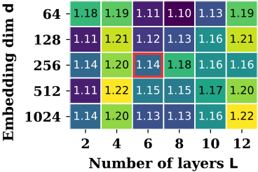
Implementation and Evaluation. We evaluated sensitivity to the main RGCL hyperparameters: the number of layers L and the embedding dimension d. Across 30 configurations spanning L ∈ {2, 4, 6, 8, 10, 12} and d ∈ {64, 128, 256, 512, 1024}, mean ECE remains within [1.10, 1.22]%, and per-configuration standard deviations fall within [0.71, 0.97]. The chosen configuration (L = 6, d = 256) achieves a mean ECE of 1.14 ± 0.74%, which reflects an arbitrary selection of hyperparameters to avoid overfitting to the evaluation data. Figure 1 summarizes the results of the mean ECE for the entire grid. Notice that the relative ranking against the baselines remains stable across the tested grid, and that the selected configuration is not optimized. All experiments were conducted on a single NVIDIA RTX 3090 GPU with 24GB VRAM and 32GB system RAM using PyTorch. We report ECE with M=15 bins, as used in [Guo et al., 2017], averaged over multiple seeds with 95% confidence intervals, as standard.
| Dataset | Model (Acc) | Uncal | TS | Platt | Isotonic | Beta | DAC | Fast Separation | TULIP | D.Ens | RGCL | RGCC |
|---|---|---|---|---|---|---|---|---|---|---|---|---|
| CIFAR10 CIFAR10 CIFAR10 CIFAR10 CIFAR10 CIFAR100 TINY | densenet121 (94.83±0.59) | 3.59±0.10 | 1.51±0.07 | 2.08±0.32 | 0.67±0.04 | 1.25±0.04 | 1.30±0.08 | 0.64±0.08 | - | 1.47±0.07 | 0.59±0.07 | 0.39±0.06 |
| resnet101 (94.44±0.15) | 4.34±0.20 | 1.34±0.12 | 2.21±0.18 | 0.82±0.07 | 1.33±0.07 | 1.10±0.09 | 0.77±0.06 | 2.50±1.12 | 2.22±0.19 | 0.69±0.07 | 0.65±0.07 | |
| resnet152 (94.37±0.15) | 4.38±0.10 | 1.46±0.06 | 2.21±0.09 | 0.77±0.06 | 1.38±0.05 | 1.06±0.06 | 0.82±0.07 | 2.60±0.50 | 1.82±0.10 | 0.72±0.06 | 0.75±0.08 | |
| resnet18 (93.84±0.67) | 3.86±0.15 | 1.60±0.10 | 2.74±0.40 | 0.92±0.06 | 1.45±0.09 | 1.19±0.09 | 0.94±0.08 | - | 3.05±0.63 | 0.81±0.10 | 0.83±0.10 | |
| resnet50 (94.15±0.49) | 3.99±0.13 | 1.42±0.07 | 2.53±0.40 | 0.80±0.05 | 1.40±0.06 | 0.92±0.05 | 0.89±0.05 | 3.00±0.24 | 1.44±0.16 | 0.67±0.05 | 0.79±0.07 | |
| CIFAR100 | densenet121 (78.91±0.24) | 13.65±0.44 | 3.75±0.16 | 8.72±0.25 | 1.99±0.21 | 5.67±0.14 | 3.52±0.13 | 1.27±0.16 | - | 4.42±0.33 | 1.36±0.18 | 1.12±0.17 |
| CIFAR100 | dinov2(L) (84.57±1.21) | 33.04±5.16 | 2.43±0.50 | 13.30±1.04 | 1.31±0.17 | 5.00±0.76 | - | 1.12±0.72 | - | - | 0.91±0.43 | 1.15±0.61 |
| CIFAR100 | resnet101 (76.83±0.33) | 11.48±0.87 | 4.41±0.12 | 7.87±0.17 | 2.06±0.12 | 5.78±0.18 | 3.77±0.10 | 1.58±0.16 | 6.71±0.10 | 4.24±0.46 | 1.49±0.15 | 1.50±0.11 |
| CIFAR100 | resnet152 (76.64±0.38) | 10.76±1.11 | 4.45±0.23 | 7.91±0.29 | 2.01±0.14 | 5.67±0.18 | 3.74±0.21 | 1.65±0.17 | 6.62±0.32 | 5.63±1.41 | 1.46±0.17 | 1.66±0.16 |
| CIFAR100 | resnet18 (75.94±0.31) | 5.51±0.43 | 3.10±0.18 | 6.90±0.15 | 1.39±0.11 | 4.56±0.19 | 3.40±0.18 | 1.54±0.22 | - | 6.27±1.64 | 1.59±0.12 | 1.57±0.30 |
| resnet50 (77.25±0.38) | 12.18±0.49 | 4.11±0.13 | 8.15±0.13 | 1.88±0.14 | 5.94±0.11 | 3.89±0.14 | 1.60±0.13 | 6.58±0.02 | 4.46±0.45 | 1.40±0.11 | 1.38±0.18 | |
| resnet101 (59.35±0.40) | 2.91±1.00 | 2.29±0.53 | 23.74±0.48 | 1.61±0.23 | 2.06±0.48 | 1.84±0.34 | 1.48±0.64 | - | 5.61±1.64 | 1.30±0.16 | 1.11±0.43 | |
| TINY | resnet152 (57.90±2.09) | 2.25±0.41 | 2.01±0.33 | 24.30±0.40 | 1.52±0.21 | 1.58±0.19 | 1.82±0.29 | 1.60±0.22 | - | 14.12±2.36 | 1.24±0.23 | 0.84±0.23 |
| TINY | resnet50 (57.46±0.37) | 3.29±0.86 | 2.42±0.35 | 23.68±0.49 | 1.60±0.50 | 2.22±0.33 | 2.07±0.22 | 1.51±0.49 | - | 5.36±1.71 | 1.32±0.53 | 0.90±0.26 |
5 Results
This section demonstrates that: (1) RGCL achieves strong top-label calibration across architectures and datasets (Section 5.1), (2) random layer sampling matches or exceeds optimized selection (Section 5.2), and (3) RGCC provides an efficient alternative with competitive results (Section 5.3).
5.1 RGCL Achieves Strong Top-Label Calibration
To evaluate the calibration performance of RGCL, we compare it against two families of single-model post-hoc calibrators. Logit-based methods: Temperature Scaling (TS) [Guo et al., 2017], Top Label Isotonic Regression [Zadrozny and Elkan, 2002; Gupta and Ramdas, 2022], Platt Scaling [Platt, 2000], and Beta Calibration [Kull et al., 2017]. Featurebased methods: Fast Separation [Chouraqui et al., 2022] (geometric separation in pixel space), DAC [Tomani et al., 2023]
(density-aware calibration with architecture-specific layers), and TULIP [Benkert et al., 2024] (layered intermediate predictions) 1 . We additionally report Deep Ensembles [Lakshminarayanan et al., 2017] as a high-cost uncertainty reference.
Table 1 shows the ECE of these algorithms on the evaluated models and datasets. As can be observed, RGCL consistently achieves the lowest or near-lowest ECE across the considered datasets and architectures. Specifically, RGCL achieves an average rank of ∼1.71 across all configurations (∼1.21 when RGCC is excluded), ranking first or second in 12 of 14 settings. Relative to uncalibrated predictions, RGCL reduces ECE by 78% on average, and by up to 97% on CIFAR100 DINOv2. Against the best non-RGC baseline, RGCL achieves an average improvement of 12% and up to 19%.
Beyond ECE. Since RGC calibrates top-label confidence [Gupta and Ramdas, 2022], ECE is our primary metric. However, we also evaluate Adaptive ECE [Nixon et al., 2019] and top-label MCE to assess whether the conclusions remain stable across related binning-based calibration metrics. On Adaptive ECE, both RGCL and RGCC achieve an average rank of approximately 1.57 against non-RGC baselines, with top-three placement in 13 and 12 out of 14 evaluated configurations, respectively. On MCE, RGCC slightly improves over RGCL in average rank (2.79 vs. 3.00), and both methods rank in the top-three in 9 of 14 configurations. We conclude that the selected metric is representative, and we obtain similar results with other metrics.
1 The experimental results for TULIP are taken directly from [Benkert et al., 2024].
| vs GC(DAC) | vs RGCC | |||||||||
|---|---|---|---|---|---|---|---|---|---|---|
| Dataset | Model | RGCL | GC(DAC) | Diff (pp) | TOST p | Result | RGCC | Diff (pp) | TOST p | Result |
| CIFAR10 | densenet121 | 0.59±0.26 | 0.58±0.19 | -0.01 | <0.001 | Eq. | 0.39±0.24 | -0.20 | <0.001 | Eq. |
| CIFAR10 | resnet101 | 0.69±0.25 | 0.67±0.22 | -0.02 | <0.001 | Eq. | 0.65±0.24 | -0.04 | <0.001 | Eq. |
| CIFAR10 | resnet152 | 0.72±0.30 | 0.66±0.30 | -0.06 | <0.001 | Eq. | 0.75±0.39 | +0.03 | <0.001 | Eq. |
| CIFAR10 | resnet18 | 0.81±0.32 | 0.81±0.40 | -0.00 | <0.001 | Eq. | 0.83±0.33 | +0.02 | <0.001 | Eq. |
| CIFAR10 | resnet50 | 0.69±0.23 | 0.67±0.24 | -0.04 | <0.001 | Eq. | 0.79±0.28 | +0.10 | <0.001 | Eq. |
| CIFAR100 | densenet121 | 1.36±0.45 | 1.29±0.27 | -0.06 | 0.007 | Eq. | 1.12±0.41 | -0.23 | 0.056 | - |
| CIFAR100 | resnet101 | 1.49±0.59 | 1.45±0.50 | -0.04 | <0.001 | Eq. | 1.50±0.45 | +0.02 | <0.001 | Eq. |
| CIFAR100 | resnet152 | 1.46±0.52 | 1.33±0.37 | -0.12 | 0.017 | Eq. | 1.66±0.46 | +0.20 | 0.014 | Eq. |
| CIFAR100 | resnet18 | 1.59±0.31 | 1.35±0.26 | -0.24 | 0.021 | Eq. | 1.57±0.75 | -0.02 | 0.011 | Eq. |
| CIFAR100 | resnet50 | 1.40±0.36 | 1.30±0.41 | -0.10 | 0.002 | Eq. | 1.38±0.57 | -0.04 | 0.009 | Eq. |
| TINY | resnet101 | 1.37±0.10 | 1.39±0.45 | +0.02 | 0.086 | - | 1.19±0.41 | -0.18 | 0.129 | - |
| TINY | resnet152 | 1.02±0.30 | 1.37±0.29 | +0.35 | 0.232 | - | 0.61±0.44 | -0.42 | 0.388 | - |
| TINY | resnet50 | 1.16±0.15 | 1.22±0.52 | +0.06 | 0.102 | - | 0.61±0.29 | -0.54 | 0.583 | - |
5.2 SamplingMatches Optimal Layer Selection
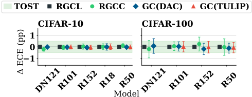
We compare RGCL and RGCC with geometric calibrators that rely on optimized layer selection, namely DAC and TULIP, denoted GC(DAC) and GC(TULIP). Figure 3 reports ECE normalized relative to RGCL. The differences cluster near zero and mostly fall within the δ = 0.5 percentagepoint equivalence band suggesting that RGCL and RGCC achieve equivalent calibration performance to carefully selecting layer configurations.
Table 2 reports the corresponding numerical results. To formally assess equivalence, we perform two one-sided tests (TOST) [Schuirmann, 1987] with margin δ=0.5 percentage points. The test establishes equivalence in 10 of 13 modeldataset configurations, and in no configuration is RGCL found to be significantly worse than DAC- or TULIP-based layer selection. Taken together, these results show that our randomized sampling strategy can replace carefully tuned layer selection without a statistically significant degradation in calibration performance.
5.3 RGCC Provides Comparable Calibration at Lower Preprocessing Cost
This section compares RGCL and RGCC using TOST equivalence testing, with results reported in Table 2. Of the 13 dataset and model combinations, 9 establish formal equivalence at margin δ = 0.5 percentage points. The point estimates mildly favor RGCL on CIFAR-10 and CIFAR-100 on average, whereas RGCC achieves lower ECE on average on Tiny-ImageNet. The remaining configurations do not establish equivalence, primarily due to higher variance or fewer paired trials. Overall, the differences are small, and combined with RGCC's lower preprocessing cost (Section 5.5), this makes RGCC an attractive option for resource-constrained deployment.
5.4 Why RGCL Works
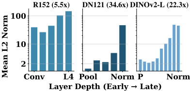
At first glance, the strong performance of RGCL and RGCC may seem surprising. Unlike prior work, our method does not rely on explicit per-layer weighting, even though uniformly weighting layers is generally suboptimal when many layers are uninformative. We show that layers exhibiting strong geometric separation also tend to have disproportionately large L2 norms. As a result, once such a layer is sampled, it naturally dominates the aggregation.
Figure 2 plots the average L2 norm of pooled feature vectors, ∥vℓ(x)∥2, across layers for three architectures on CIFAR-100. We observe a consistent increase in norm magnitude from early to late layers: 5.5× for ResNet-152, 22.3× for DINOv2-Large (despite a constant embedding dimension), and 34.6× for DenseNet-121 (likely driven by dense feature concatenation). In DINOv2-Large, the embedding dimension is fixed, and we still see larger norms in important layers. When projected vectors are summed, layers with larger norms therefore contribute disproportionately to the induced Euclidean geometry, effectively emphasizing later blocks without requiring explicit layer weighting. We emphasize that this is an empirical explanation rather than a worstcase guarantee: in architectures where late-layer norms do not dominate, the implicit weighting effect may be weaker or distributed more uniformly across layers.
This implicit emphasis on a small number of informative layers motivates the second design choice of our method. Once the layers are selected, we compress them into a compact representation with drastically fewer coordinates. The effectiveness of this compression is consistent with growing evidence that learned representations exhibit substantial distributed redundancy. For example, Nanda et al. [Nanda et al., 2023] demonstrate that randomly selected neuron subsets preserve much of a layer's representational power.
5.5 Computational Efficiency
In this section, we evaluate the computational overhead of our proposed methods. We consider two benchmarks: the offline preprocessing time and the online inference throughput.
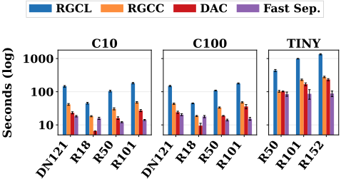
First, we evaluate the offline preprocessing time required by our methods. These results are shown in Figure 4. As expected, RGCL requires more preprocessing time than the alternative methods. RGCC substantially reduces this cost; however, the preprocessing time remains higher than that of prior work. This overhead constitutes a limitation of our approach, but it is incurred only once during calibration setup and does not affect inference-time performance.
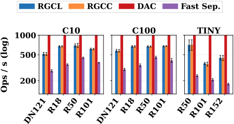
Second, we evaluate the number of confidence estimates produced per second on each dataset. Figure 5 reports these results. We observe that DAC is considerably faster than both RGCL and RGCC. The two variants attain nearly identical inference speeds, as they execute the same geometric scoring procedure on slightly different feature representations. Fast Separation [Chouraqui et al., 2022] is slower still, and its throughput depends directly on the input dimensionality. In contrast, our methods project inputs into a fixed-dimensional random subspace, yielding a constant computational cost independent of the original input size.
The main takeaway from these experiments is the tradeoff inherent in our approach and in geometric calibration methods more broadly. Unlike purely logit-based calibrators, RGCL and RGCC require an offline preprocessing stage for feature extraction and nearest-neighbor index construction, which can be costly when the calibration set or data distribution changes frequently. However, once this index is built, both variants support several hundred confidence estimates per second, making them compatible with real-time vision workloads such as video-rate inference. Thus, RGC is best suited to settings with relatively stable calibration data, where improved top-label calibration justifies additional offline preprocessing and moderate online overhead.
6 Discussion
Our work contributes to the ongoing line of research on geometric confidence calibration. We demonstrate that explicit layer selection and weighting can be avoided by adopting layer-based or coordinate-based sampling schemes, and that the dimensionality of the geometric feature space can be drastically reduced without sacrificing performance. These findings reinforce observations by Nanda et al. [Nanda et al., 2023] regarding the high degree of redundancy present in late-stage feature representations.
Building on these insights, we introduce a geometric confidence calibration method. The method assesses how close an input representation lies to the boundary of the class-induced geometry.
We further show that our approach outperforms several recently proposed geometric confidence calibrators, including DAC [Tomani et al., 2023], TULIP [Benkert et al., 2024], and Separation [Chouraqui et al., 2022], establishing a strong empirical contribution to the literature on confidence estimation. Through extensive evaluation, we analyze both the strengths and limitations of our method, provide insight into its effectiveness, and position its computational overhead within the broader literature, exposing the trade-offs involved.
Our evaluation is limited to in-distribution imageclassification benchmarks.
Evaluating RGC under corruptions, domain shift, and nonvision modalities is an important direction for future work.
Looking forward, our results suggest that future geometric calibrators may benefit from placing less emphasis on explicit layer selection and weighting. Such design choices can introduce additional adaptivity to specific architectures or datasets, potentially limiting transfer across models. In contrast, randomized sampling strategies, such as the two variants proposed in this work, offer a simple and architecture-agnostic route for constructing informative geometric feature spaces.
An additional promising direction is the approximation of reduced semantic feature spaces induced by successful geometric calibrators using smaller neural networks. We hypothesize that such networks could produce embeddings better suited for semantic caching, potentially leading to improved efficiency and performance.
@inproceedings{ijcai2026p458,
  title     = {Semantic Geometric Calibration in Randomized Neural Feature Space},
  author    = {Abuhazera, Itay and Cohen, Liron and Einziger, Gil},
  booktitle = {Proceedings of the Thirty-Fifth International Joint Conference on
               Artificial Intelligence, {IJCAI-26}},
  publisher = {International Joint Conferences on Artificial Intelligence Organization},
  editor    = {Diego Calvanese},
  pages     = {4116--4124},
  year      = {2026},
  month     = {8},
  note      = {Main Track},
  doi       = {10.24963/ijcai.2026/458},
  url       = {https://doi.org/10.24963/ijcai.2026/458},
}
TY - CPAPER TI - Semantic Geometric Calibration in Randomized Neural Feature Space AU - Abuhazera, Itay AU - Cohen, Liron AU - Einziger, Gil T2 - Proceedings of the Thirty-Fifth International Joint Conference on Artificial Intelligence, IJCAI-26 PB - International Joint Conferences on Artificial Intelligence Organization PY - 2026 SP - 4116 EP - 4124 DO - 10.24963/ijcai.2026/458 UR - https://doi.org/10.24963/ijcai.2026/458 ER -Copied
Machine-readable versions of this paper, for tools and AI agents:





