
Interference-free Walks in Time: Temporally Disjoint Paths
Proceedings of the Thirtieth International Joint Conference on Artificial Intelligence. Main Track. Pages 4090-4096.
https://doi.org/10.24963/ijcai.2021/563
Keywords
- Agent-based and Multi-agent Systems: Multi-agent Planning
- Planning and Scheduling: Planning and Scheduling
- Planning and Scheduling: Scheduling
Abstract
We investigate the computational complexity of finding temporally disjoint paths or walks in temporal graphs. There, the edge set changes over discrete time steps and a temporal path (resp. walk) uses edges that appear at monotonically increasing time steps. Two paths (or walks) are temporally disjoint if they never use the same vertex at the same time; otherwise, they interfere. This reflects applications in robotics, traffic routing, or finding safe pathways in dynamically changing networks.
On the one extreme, we show that on general graphs the problem is computationally hard. The "walk version" is W[1]-hard when parameterized by the number of routes. However, it is polynomial-time solvable for any constant number of walks. The "path version" remains NP-hard even if we want to find only two temporally disjoint paths. On the other extreme, restricting the input temporal graph to have a path as underlying graph, quite counterintuitively, we find NP-hardness in general but also identify natural tractable cases.
- [Almagor and Lahijanian, 2020] S. Almagor and M. Lahija- nian. Explainable multi agent path finding. In AAMAS, pages 34-42, 2020.
- [Atzmon et al., 2020] D. Atzmon, R. Stern, A. Felner, G. Wagner, R. Barták, and N.-Fa Zhou. Robust multi-agent path finding and executing. J. Artif. Intell. Res., 67:549- 579, 2020.
- [Bentert et al., 2020] M. Bentert, A.-S. Himmel, A. Nich- terlein, and R. Niedermeier. Efficient computation of opti- mal temporal walks under waiting-time constraints. Appl. Netw. Sci., 5(1):73, 2020.
- [van Bevern et al., 2015] R. van Bevern, M. Mnich, R. Nie- dermeier, and M. Weller. Interval scheduling and colorful independent sets. J. Sched, 18(5):449-469, 2015.
- [Bollobás, 1986] B. Bollobás. Combinatorics: Set Sys- tems, Hypergraphs, Families of Vectors, and Combinato- rial Probability. Cambridge University Press, 1986.
- [Casteigts et al., 2020] A. Casteigts, A.-S. Himmel, H. Mol- ter, and P. Zschoche. The computational complexity of finding temporal paths under waiting time constraints. In ISAAC, pages 30:1-30:18, 2020.
- [Chuzhoy et al., 2017] J. Chuzhoy, D.H.K. Kim, and R. Ni- mavat. New hardness results for routing on disjoint paths. In STOC, pages 86-99, 2017.
- [Dondi and Sikora, 2017] R. Dondi and F. Sikora. Finding disjoint paths on edge-colored graphs: more tractability results. J. Comb. Optim., 36:1315-1332, 2017.
- [Downey and Fellows, 2013] R.G. Downey and M.R. Fel- lows. Fundamentals of Parameterized Complexity. Texts in Computer Science. Springer, 2013.
- [Enright et al., 2021] Jessica Enright, Kitty Meeks, George B. Mertzios, and Viktor Zamaraev. Deleting edges to restrict the size of an epidemic in temporal networks. J. Comput. Syst. Sci., 119:60-77, 2021.
- [Fluschnik et al., 2019a] T. Fluschnik, S. Kratsch, R. Nieder- meier, and M. Sorge. The parameterized complexity of the minimum shared edges problem. J. Comput. Syst. Sci., 106:23-48, 2019.
- [Fluschnik et al., 2019b] T. Fluschnik, M. Morik, and M. Sorge. The complexity of routing with collision avoid- ance. J. Comput. Syst. Sci., 102:69-86, 2019.
- [Fortune et al., 1980] S. Fortune, J. Hopcroft, and J. Wyllie. The directed subgraph homeomorphism problem. Theor. Comput. Sci., 10(2):111-121, 1980.
- [Golovach and Thilikos, 2011] P.A. Golovach and D.M. Thi- likos. Paths of bounded length and their cuts: parameter- ized complexity and algorithms. Discrete Optim., 8(1):72- 86, 2011.
- [Guo et al., 2018] L. Guo, Y. Deng, K. Liao, Q. He, T. Sellis, and Z. Hu. A fast algorithm for optimally finding partially disjoint shortest paths. In IJCAI, pages 1456-1462, 2018. IJCAI
- [Karp, 1975] R.M. Karp. On the computational complexity of combinatorial problems. Networks, 5(1):45-68, 1975.
- [Kawarabayashi et al., 2012] K. Kawarabayashi, Y. Kobaya- shi, and B. Reed. The disjoint paths problem in quadratic time. J. Comb. Theory, Ser. B, 102(2):424-435, 2012.
- [Kempe et al., 2002] D. Kempe, J. Kleinberg, and A. Ku- mar. Connectivity and inference problems for temporal networks. J. Comput. Syst. Sci., 64(4):820-842, 2002.
- [Klobas et al., 2021] Nina Klobas, George B. Mertzios, Hendrik Molter, Rolf Niedermeier, and Philipp Zschoche. Interference-free walks in time: Temporally disjoint paths. CoRR, abs/2105.08335, 2021.
- [Mertzios et al., 2019] G.B. Mertzios, O. Michail, and P.G. Spirakis. Temporal network optimization subject to con- nectivity constraints. Algorithmica, 81(4):1416-1449, 2019.
- [Robertson and Seymour, 1985] N. Robertson and P.D. Sey- mour. Disjoint paths-a survey. SIAM J. Algebraic Dis- crete Methods, 6(2):300-305, 1985.
- [Robertson and Seymour, 1995] N. Robertson and P.D. Sey- mour. Graph minors. XIII. The disjoint paths problem. J. Comb. Theory, Ser. B, 63(1):65-110, 1995.
- [Santos et al., 2017] R.F. Santos, A. Andrioni, A.C. Drum- mond, and E.C. Xavier. Multicolour paths in graphs: NP- hardness, algorithms, and applications on routing in WDM networks. J. Comb. Optim., 33(2):742-778, 2017.
- [Slivkins, 2010] A. Slivkins. Parameterized tractability of edge-disjoint paths on directed acyclic graphs. SIAM J. Discrete Math., 24(1):146-157, 2010.
- [Standley, 2010] T.S. Standley. Finding optimal solutions to cooperative pathfinding problems. In AAAI, pages 173- 178, 2010.
- [Stern et al., 2019] R. Stern, N.R. Sturtevant, A. Felner, S. Koenig, H. Ma, T.T. Walker, J. Li, D. Atzmon, L. Co- hen, T.K.S. Kumar, R. Barták, and E. Boyarski. Multi- agent pathfinding: Definitions, variants, and benchmarks. In SOCS, pages 151-159, 2019.
- [Stern, 2019] R. Stern. Multi-agent path finding -an overview. In Artificial Intelligence -5th RAAI Summer School, pages 96-115. Springer, 2019.
- [Tao et al., 2020] B. Tao, M. Xiao, and J. Zhao. Finding minimum-weight link-disjoint paths with a few common nodes. In AAAI, pages 938-945, 2020.
- [Tovey, 1984] C.A. Tovey. A simplified NP-complete satis- fiability problem. Discrete Appl. Math., 8(1):85-89, 1984.
- [Wu et al., 2016] H. Wu, J. Cheng, Y. Ke, S. Huang, Y. Huang, and H. Wu. Efficient algorithms for tempo- ral path computation. IEEE Trans. Knowl. Data Eng., 28(11):2927-2942, 2016.
- [Wu, 2012] B.Y. Wu. On the maximum disjoint paths prob- lem on edge-colored graphs. Discrete Optim., 9(1):50-57, 2012.
References were extracted automatically from the PDF and may contain errors.
Full text extracted automatically from the PDF; figures, tables and equations may differ. The PDF is the version of record.
1 Introduction
Computing (vertex-)disjoint paths in a graph is a cornerstone problem of algorithmic graph theory. One of the deepest achievements in discrete mathematics, graph minor theory [Robertson and Seymour, 1985; Robertson and Seymour, 1995], as well as the theory of parameterized complexity analysis [Downey and Fellows, 2013] are tightly connected to it. The problem is known to be solvable in quadratic time if the number of paths is constant, that is, it is fixedparameter tractable when parameterized by the number of paths [Kawarabayashi et al., 2012]. Besides being of fundamental interest in (algorithmic) graph theory, finding disjoint paths has many applications and there exist numerous variations of the problem. In AI and robotics scenarios, for instance, multi-agent path finding is an intensively studied, closely related problem [Stern, 2019; Stern et al., 2019].
∗ Supported by the EPSRC grant EP/P020372/1 and by DFG RTG 2434 while visiting TU Berlin.
†Supported by the German Research Foundation (DFG), project MATE (NI 369/17), and by the Israeli Science Foundation (ISF), grant No. 1070/20. The main part of this work was done while the author was affiliated with TU Berlin.

Coming from the graph-algorithmic side, we propose a new view on finding disjoint paths (and walks), that is, we place the problem into the world of temporal graphs. We add a "new dimension" to the classic, static graph scenario by generalizing to a setting where the edges of a graph may appear and disappear over (discrete) time. In our model, we consider two paths (or walks) to be disjoint if they do not use the same vertex at the same point of time. Consider Fig. 1 for an example. Moreover, the path finding also has to take into account that edges are not permanently available, reflecting dynamic aspects of many real-world scenarios such as routing in traffic or communication networks, or the very dynamic nature of social networks. We intend to initiate studies on this natural scenario. Doing so, we focus on two extreme cases for the underlying graphs, namely the (underlying) graph structure being completely unrestricted or it being restricted to just a path graph. For these opposite poles, performing (parameterized) computational complexity studies, we present surprising discoveries. Before coming to these, we discuss (excerpts of) the large body of related work.
1.1 RelatedWork
As said, both the literature on (static) disjoint paths and its many variants as well as on multi-agent path finding is very rich. Hence, we only list a small fraction of the relevant related work. In context of graph-algorithmic work, the polynomial-time (in-)approximability of the NP-hard maximization version has been studied [Chuzhoy et al., 2017]. Variants of the basic problem studied include bounds on the path length [Golovach and Thilikos, 2011] or relaxing on the disjointness of paths [Fluschnik et al., 2019a;
Fluschnik et al., 2019b; Guo et al., 2018; Tao et al., 2020].
In directed graphs, finding two disjoint paths is already NPhard [Fortune et al., 1980], whereas in directed acyclic graphs the problem is solvable in polynomial time for every fixed number of paths [Slivkins, 2010].
As to multi-agent path planning, we remark that it has been intensively researched (with several possible definitions) in the last decade in the AI and robotics communities [Almagor and Lahijanian, 2020; Atzmon et al., 2020; Standley, 2010; Stern, 2019; Stern et al., 2019]. Timing issues (concurrency of moving agents) or various objective functions of the agents play a fundamental role here, and also a high variety of conflict scenarios is studied. 1 The scenario we study in this work can be interpreted as a basic variant of multi-agent path planning, now translated into the world of temporal graphs.
In algorithmic graph theory, also edge-colored graphs are studied. Edge-colored graphs essentially are multilayer (or multiplex) graphs where the essential difference to temporal graphs is that there is no order on the graph layers. Here, pathfinding scenarios are e.g. motivated by applications in social and optical (routing) networks [Dondi and Sikora, 2017; Santos et al., 2017; Wu, 2012].
Finally, as to temporal graphs, note that several prominent graph problems have been studied in this fairly new framework. This particularly includes research on path problems [Bentert et al., 2020; Enright et al., 2021; Casteigts et al., 2020; Mertzios et al., 2019; Wu et al., 2016]. In particular, another model of vertex-disjoint temporal paths [Kempe et al., 2002], where two temporal paths are considered vertexdisjoint if they do not visit the same vertex. The problem of finding two such paths is NP-hard [Kempe et al., 2002]. Note that the major difference to our model is that we allow two temporally disjoint paths to visit the same vertex as long as they do not both visit that vertex at the same time.
Our contributions. Our results can be grouped into two parts. First, studying temporal graphs where the underlying graph (which is obtained by making all temporal edges permanent) is unrestricted, we show that finding walks instead of paths turns out to be computationally easier. More specifically, finding temporally disjoint walks is W[1]-hard with respect to the number of walks but can be solved in polynomial time if this number is constant (i.e., we develop an XP algorithm), whereas finding temporally disjoint paths already turns out to be NP-hard for two paths. Second, restricting the input to be a temporal line (i.e., the underlying graph to be a path), we find a polynomial-time algorithm for a relevant special case while the problem remains NP-hard in general (for both paths and walks). However, we also provide a fixed-parameter tractability result with respect to the number of paths. We survey our results in Table 1. Due to space constraints, proofs of results marked with ⋆ are (partially) deferred to a full version on arXiv [Klobas et al., 2021].
2 Preliminaries and ProblemDefinition
We denote by N and N0 the natural numbers excluding and including 0, respectively. An interval on N0 from a to b is denoted by [a, b] := {i ∈ N0 | a ≤ i ≤ b} and [a] := [1, a].
1 Also see http://mapf.info/
| TEMP. DISJOINT | PATHS | WALKS |
| unrestricted underlying graph | NP-hard for |S| = 2 | W[1]-hard wrt. |S| XP wrt. |S| |
| temporal line or tree | NP-hard FPT wrt. |S| open | |
| temporal line & S contains only pairs of extremal points | poly-time | |
Static graphs. An undirected graphG = (V,E) consists of a set V of vertices and a set E ⊆ {{v, w} | v, w ∈ V, v ̸= w} of edges. For a graph G, we also denote by V (G) and E(G) the vertex and edge set of G, respectively. A path P = (V, E) is a graph with a set V (P ) = {v1, . . . , vk} of distinct vertices and edge set E(P) = {{vi, vi+1} | 1 ≤ i < k} (we often represent path P by the tuple (v1, v2, . . . , vk)). We say that P is a (v1, vk)-path and that P visits all vertices in V (P).
A temporal graph G = (V, (Ei)i∈[T]) consists of a set V of vertices and lifetime T many edge sets E1,E2, . . . ,ET over V . The pair (e, i) is a time edge of G if e ∈ Ei. The graph (V,Ei) is called the i-th layer of G. The underlying graph of G is the static graph (V, ⋃Ti=1 Ei). A temporal (s, z)-walk (or temporal walk from s to z) of length k from vertex s = v0 to vertex z = vk in G is a sequence P = ((vi-1, vi, ti))ki=1 of triples such that for all i ∈ [k] we have that {vi-1, vi} ∈ Eti and for all i ∈ [k - 1] we have that ti ≤ ti+1. The arrival time of P is tk. We say that P visits the vertices V (P) := {vi | i ∈ [0, k]}. In particular, P visits vertex vi during the time interval [ti, ti+1], for all i ∈ [k - 1]. Furthermore, we say that P visits v0 during time interval [t1, t1] and P visits vk during time interval [tk, tk]. A temporal (s, z)-walk P = ((vi-1, vi, ti))ki=1 of length k is called a temporal (s, z)-path (or temporal path from s to z) if vi ̸= vj whenever i ̸= j. Given two temporal walks P1, P2 we say that P1 and P2 temporally intersect if there exists a vertex v and two time intervals [a1, b1], [a2, b2], where [a1, b1] ∩ [a2, b2] ̸= ∅, such that v is visited by P1 during [a1, b1] and by P2 during [a2, b2]. Now, we can formally define our problem.
TEMPORALLY DISJOINT PATHS
Input: A temporal graph G = (V, (Ei)i∈[T]) and a multiset S of source-sink pairs containing elements from V × V .
Question: Are there pairwise temporally nonintersecting temporal (si, zi)-paths for all (si, zi) ∈ S?
Analogously, TEMPORALLY DISJOINT WALKS gets the same input but asks whether there are pairwise temporally non-intersecting temporal (si, zi)-walks for all (si, zi) ∈ S. From the NP-hardness of DISJOINT PATHS [Karp, 1975], we immediately get the following.
Observation 1. TEMPORALLY DISJOINT (PATHS/WALKS) is NP-hard even if T = 1.
By potentially applying a linear-time preprocessing step to the input, we may assume without loss of generality that all edge sets Ei, i = 1, 2, . . . , T , are non-empty. Hence, the size of G is |G| := |V | + ∑Tt=1 |Et|.
Parameterized complexity. Let Σ denote a finite alphabet. A parameterized problem L ⊆ {(x, k) ∈ Σ∗ × N0} is a subset of all instances (x, k) from Σ∗ × N0, where k denotes the parameter. A parameterized problem L is (i) FPT (fixedparameter tractable) if there is an algorithm that decides every instance (x, k) for L in f(k) · |x|O(1) time, and (ii) contained in the class XP if there is an algorithm that decides every instance (x, k) for L in |x|f(k) time. where f is any computable function only depending on the parameter. If a parameterized problem L is W[1]-hard, then it is presumably not fixed-parameter tractable.
3 The Case of Few Source-Sink Pairs
In this section, we study the computational complexity of TEMPORALLY DISJOINT (PATHS/WALKS) for the case that the size of the multiset S of source-sink pairs is small. We start by showing that TEMPORALLY DISJOINT PATHS is NPhard even for two sink-source pairs. This is a similar situation as for finding vertex-disjoint paths in directed static graphs, which is also NP-hard for two paths [Fortune et al., 1980]. However, in the temporal setting there is a surprising difference between finding walks and paths that does not have an analogue in the static setting. We show that TEMPORALLY DISJOINT WALKS is W[1]-hard for the number |S| of sourcesink pairs and is contained in XP for the same parameter.
Theorem2. [⋆] TEMPORALLY DISJOINT PATHS is NP-hard even if |S| = 2 and T = 3.
Proof sketch. We show that TEMPORALLY DISJOINT PATHS is NP-hard even if |S| = 2 and T = 3 by a polynomialtime reduction from the NP-complete EXACT (3, 4)-SAT problem [Tovey, 1984]. EXACT (3, 4)-SAT asks whether a Boolean formula φ is satisfiable, assuming that it is in conjunctive normal form, each clause has exactly three literals, and each variable appears in exactly four clauses.
Let φ be an instance of EXACT (3, 4)-SAT with n variables x1, x2, . . . , xn and m clauses. We construct an instance I = (G = (V, (E1, E2, E3)), S = {(s1, z1), (s2, z2)}) in the following way. Intuitively, the first two layers contain the assignment gadget for the variables. The part of the temporal (s1, z1)-path P1 which is in the first layer sets all variables. The temporal (s2, z2)-path ensures that P1 does not "wait" in a variable gadget. In the third layer, P1 must go from s′ to z1 through all clause gadgets. Since P1 cannot visit a vertex twice, this validates whether the assignment satisfies φ. Fig. 2 depicts the resulting temporal graph.
The construction is done as follows. For each variable xj we construct the variable gadget G xj = ({axj , axj+1 } ∪ {xj i , xj i | i ∈ [4]}, (Exj i )i∈[2]), where Exj 1 = Exj T ∪ Exj F with Exj T = {{axj , xj 1 }, {xj 4 , axj+1 }}∪{{xj i , xj i+1 } | i ∈ [3]} and Exj F = {{axj , xj 1 }, {xj 4 , axj+1 }} ∪ {xj i , xj i+1 |
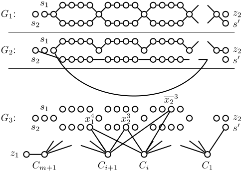
i ∈ [3]}, and Exj 2 = Exj T ∪ {{xj i , xj i+1 } | i ∈ [3]} ∪ {{xj 4 , xj+1 1 } | j < n}. Let Ci = (ℓfj ∨ℓgp ∨ℓhq ) be a clause, where ℓβα is a literal of variable xα and its β-th appearance when iterating the clauses in the order of the indices. We now abuse our notation and say ℓβα ≡ xβα if ℓβα is a negation of xα and otherwise we say ℓβα ≡ xβα. We construct the clause gadget G Ci := ({Ci,Ci+1, ℓfj , ℓgp , ℓhq }, (ECi t )t∈[3]) where ECi 1 = ECi 2 = ∅ and ECi 3 = {{Cr, ℓfj }, {Cr, ℓgp }, {Cr, ℓhq } | r ∈ {i, i + 1}}. Now we set G = (V, (Et)t∈[3]), where V = ⋃nj=1 V (G xj ) ∪ ⋃mi=1 V (G Ci ) ∪ {s1, s2, z1, z2, s′ }, E1 = ⋃nj=1 Exj 1 ∪ {{s1, ax1 }, {axn+1 , s′ }}, E2 = ⋃nj=1 Exj 2 ∪ {{s2, x1 1 }, {xn 4 , ax1 }, {axn+1 , z2}}, and E3 = ⋃mi=1 ECi 4 ∪ {{s′ , C1}, {z1, Cm+1}}.
Observe that I can be constructed in polynomial time.
The reduction behind Theorem 2 heavily relies on the fact that we are dealing with paths. Indeed, for temporally disjoint walks we presumably cannot obtain NP-hardness for a constant number of sink-source pairs since, as we will show at the end of this section, TEMPORALLY DISJOINT WALKS can be solved in polynomial time if the number of source-sink pairs is constant. However, before that we show W[1]-hardness for TEMPORALLY DISJOINT WALKS parameterized by the number |S| of source-sink pairs, presumably excluding the existence of an FPT-algorithm for this parameter.
Theorem 3. [⋆] TEMPORALLY DISJOINT WALKS is W[1]- hard when parameterized by |S|, even if all edges have exactly one time label.
We now show that TEMPORALLY DISJOINT WALKS is in XP for the parameter number |S| of source-sink pairs.
Theorem 4. [⋆] TEMPORALLY DISJOINT WALKS is in the class XP when parameterized by |S|, as it can be solved in O(|V |2|S|+2 · T) time if |S| is a fixed constant.
Proof sketch. Consider an instance I = (G, S = {(s1, z1), (s2, z2), . . . , (sk, zk)}) of TEMPORALLY DISJOINT WALKS. We use the following dynamic programming table D with Boolean entries. Intuitively, we want that for all t ∈ {1, . . . , T} and v1, . . . , vk ∈ V we have that D[t, v1, . . . , vk] = ⊤ if and only if there are temporally nonintersecting temporal (si, vi)-walks P1, . . . , Pk with arrival time ti ≤ t. However, for technical reasons, we have slightly stronger requirements for D. First of all, we have a "dummy" time label zero that we use to encode the sources in the dynamic program. Formally, we initialize D as follows:
For all v1, . . . vk ∈ V we have that
Furthermore, we have to model that the temporal walks we are looking for do not have to start immediately at their respective sources. Hence, if a temporal walk is still "waiting" at its source, the source vertex is not "blocked" for other temporal walks. We have a symmetric situation if temporal walks already arrived at their respective sink. In other words, if we have an entry D[t, v1, . . . , vk] with vi = vj for some i ̸= j, then it is a necessary condition for D[t, v1, . . . , vk] = ⊤ that at least one of the two temporal walks i, j is either still waiting at its source or already arrived at its sink. In the latter case, we additionally need that the temporal walk arrived at the sink in a previous time step, otherwise the sink would still be blocked. We now look up in D whether there all these conditions are met for a set of temporally disjoint walks that arrive at some vertices at time t - 1 such that they can be extended in time step t to reach the vertices v1, . . . , vk.
Formally, for all t ∈ [T] we have that
Here, DISJ. PATHS is the DISJOINT PATHS problem, where we are given an undirected graph G and set of k terminal pairs {(s′i , z′i ) | i ∈ [k]} and ask whether there are k vertex-disjoint paths P1, . . . , Pk in G such that Pi is an (s′i , z′i )-path and Pi and Pj are vertex-disjoint for all i ∈ [k] and j ∈ [k] \ {i}. Note that s′i = z′i is a valid input and that in this case s′i is the only vertex on an (s′i , z′i )-path. We report that I is a yesinstance if and only if D[T, z1, . . . , zk] = ⊤.
Finally, we point out that Theorem 2 implies that for TEMPORALLY DISJOINT PATHS we presumably cannot achieve a result similar to Theorem 4 while Theorem 3 implies that we presumably cannot improve this result on a classification level, that is we cannot expect to find an FPT-algorithm for TEMPORALLY DISJOINT WALKS for parameter |S|.
4 Temporal Lines and Trees
In this section, we investigate the computational complexity of TEMPORALLY DISJOINT (PATHS/WALKS) for restricted classes of underlying graphs, in particular so-called temporal lines and temporal trees. The former are temporal graphs that have a path as underlying graph and the latter are temporal graphs that have a tree as underlying graph. In particular, we first show that, surprisingly, the problems remain NP-hard on temporal lines (and thus also on temporal trees). On the positive side we show that, on temporal trees, the TEMPORALLY DISJOINT PATHS is fixed-parameter tractable with respect to the number of source-sink pairs. The latter result stands in stark contrast to the general case, where the problem is NPhard even when the number of source-sink pairs is two (Theorem 2). If we further restrict all source-sink pairs to consist of the two end-points of the temporal line, then we obtain a polynomial-time algorithm.
Before we proceed with our results in this section, first we recall some background on foremost temporal paths. Given a temporal graph G and two specific vertices s, z of it, a foremost temporal path from s to z starting at time t is a temporal path which starts at s not earlier than at time t and arrives at z with the earliest possible arrival time. A foremost temporal path from s to z starting at time t can be computed in linear O (|V | + ∑Ti=1 |Ei|) time [Wu et al., 2016].
Theorem 5. [⋆] TEMPORALLY DISJOINT (PATHS/WALKS) is NP-hard even on a temporal line where all temporal paths are to the same direction.
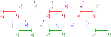
Proof sketch. We present here a polynomial-time reduction for TEMPORALLY DISJOINT WALKS. The reduction is done fromMULTICOLORED INDEPENDENT SET ON UNIT INTERVAL GRAPHS, which is known to be NP-complete [van Bevern et al., 2015, Lemma 2]. In this problem the input is a unit interval graph G = (V,E) with n vertices, where V is partitioned into k subsets of independent vertices; we interpret each of these subsets as a vertex color. The goal is to compute an independent set of size k in G which contains exactly one vertex from each color. By possibly slightly shifting the endpoints of the intervals in the given unit interval representation of G, we can assume without loss of generality that all endpoints of the intervals are distinct. Furthermore, we can assume without loss of generality that each interval endpoint is an integer between k + 1 and k + n2 (while all intervals still have the same length).
From the given multi-colored unit intervals in G, we construct a temporal line P using the following procedure. Let {c1, . . . , ck} be a set of all colors of the intervals in G. First we fix an arbitrary linear ordering c1 < c2 < . . . < ck of the k colors, and we add to the underlying path P of P two vertices v1 i and v2 i , for every color ci. We add to P also three basis vertices vℓ, v⋆ , vr. The vertices of P are ordered starting from v1 1 , v1 2 , . . . , v1 k , followed by the basis vertices vℓ, v⋆ , vr, and finishing with v2 1 , v2 2 , . . . , v2 k . At the end we have P = (v1 1 , v1 2 , . . . , v1 k , vℓ, v⋆ , vr, v2 1 , v2 2 , . . . , v2 k ).
We construct the multiset S of source-sink pairs as follows. Let mi be the number of intervals of color ci. For every
(a) Instance of the multicolored unit interval problem.
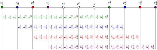
Figure 3: Example of the reduction described in the proof of Theorem 5.
color ci we add the pair (v1 i , v2 i ) to S. We refer to this sourcesink pair as "the verification source-sink pair for color ci". Furthermore, we add mi - 1 copies of the pair (v1 i , vℓ) to S and we add mi - 1 copies of pair (vr, v2 i ) to S. We call these 2mi - 2 source-sink pairs the "dummy source-sink pairs for color ci".
To fully define the temporal line P, we still need to add time labels to the edges of P. Denote by aji and bji the start and end points of the jth interval of color ci. We set up the edge labels of the path P from v1 i to v2 i as follows. To edge {v1 s , v1 s+1 } with s ∈ [k - 1] we add the labels aji with i ≤ s. To edges {v1 k , vℓ} and {vℓ, v⋆ } we add all labels aji . To edge {v2 s , v2 s+1 } with s ∈ [k - 1] we add the labels bji with i > s. To edges {v⋆ , vr} and {vr, v2 1 } we add all labels bji . See Fig. 3 for an example. The construction can clearly be performed in polynomial time.
We present here the sufficiency part.
(⇐): Assume we have a set of pairwise temporally disjoint walks for all source-sink pairs in S. Note that all edges except {vℓ, v⋆ } and {v⋆ , vr} have as many time labels as temporal walks that need to go through them. Furthermore, note that {vℓ, v⋆ } has the same labels as {v1 k , vℓ} and {v⋆ , vr} has the same labels as {vr, v2 1 }. This in particular implies that all temporal walks are in fact paths since the only vertex that could be visited by a path for more than one time step is v⋆ . Therefore, for every pair (s, z) ∈ S, no temporal path from s to z can ever stop and wait at any vertex different from v⋆ . Furthermore, the only paths going through vertex v⋆ are the paths connecting vertices v1 i and v2 i (which correspond to color ci); we will refer to this path as the color path of ci. Consider color c1 and its dummy source-sink pairs (v1 1 , vℓ). By construction, the edge {v1 1 , v1 2 } has time labels corresponding to the start points aj1 of intervals from the m1 vertices of G that have color c1. It follows that the temporal paths for these dummy source-sink pairs and the color path of c1 use only time labels corresponding to the start points aj1 of intervals from the m1 vertices of G that have color c1 until they are at vℓ or arrive at v⋆ , respectively, since they cannot wait at any vertex. Now by induction, this holds for all other colors ci and by an analogous argument, this also holds for the "second half". More specifically, we also have that temporal paths for the dummy source-sink pairs (vr, v2 i ) as well as the "second part" of the color path of ci use time labels corresponding to end points bji of intervals from the vertices of G that have color ci when going from vr (respectively v⋆ ) to their corresponding destinations.
It follows that each color path can enter and leave vertex v⋆ only at the time corresponding to the start and end points of its color intervals. In any other case some of the other vertices are blocked, which prevents the completion of others temporal S-paths. Recall that intervals of the same color are nonoverlapping. Hence, for every color path corresponding to a color ci we can find one interval [aji , bji ] such that the color path visits v⋆ in an interval that includes [aji , bji ]. Since the color paths are temporally non-intersecting, the vertices corresponding to the intervals form a multicolored independent set in G.
Next, we show fixed-parameter tractability of TEMPORALLY DISJOINT PATHS parameterized by the number |S| of source-sink pairs if the underlying graph is a tree.
Theorem 6. [⋆] TEMPORALLY DISJOINT PATHS on temporal trees is in FPT when parameterized by |S|, as it can be solved in O (|S||S|+3 · |G|) time.
Proof sketch. Let I = (G, S) be an instance of TEMPORALLY DISJOINT PATHS, the underlying graph G being a tree and S consists of k source-sink pairs (s1, z1), . . . , (sk, zk). We solve I using the following procedure.
First we can observe that, since G is a tree, every sourcesink pair (si, zi) in S corresponds to exactly one path Pi in G. Furthermore, if two paths P1 and P2 intersect in a tree, their intersection P1 ∩ P2 is a continuous path in G (potentially containing only one vertex). In the case that P1, P2 intersect, there are two ways that P1 ∩ P2 can be traversed: either first by P1 and then P2, or vice-versa. The main idea of our algorithm is that we enumerate all possible ways to traverse the intersections of each pair of paths corresponding to two source-sink pairs.
Note that the set of k paths in the tree G (where every path corresponds to one source-sink pair) have the Helly property [Bollob´as, 1986]. That is, for any three of these paths Pi, Pj, Pℓ, if they pairwise have a non-empty intersection then Pi ∩ Pj ∩ Pℓ ̸= ∅. Therefore, in order to enumerate all possible ways to traverse the intersections of each pair of source-sink paths, it suffices to just enumerate all permutations of these k paths.
We remark that it remains open whether a similar result can be obtained for TEMPORALLY DISJOINT WALKS, since we cannot assume w.l.o.g. that the temporally disjoint walks are actually paths, even on temporal lines (for an example see Fig. 4). Presumably (and in contrast to the general case) the walk version is computationally more difficult than the path version of our problem on temporal paths and trees.

Finally, we show that we can solve TEMPORALLY DISJOINT (PATHS/WALKS) in polynomial time if the underlying graph is a path and all source-sink pairs consist of the endpoints of that path.
Theorem 7. [⋆] Let G be a temporal line having P = (v0, v1, v2, . . . , vn) as its underlying path. If S contains k times the source-sink pair (v0, vn) and ℓ = |S| - k times the source-sink pair (vn, v0), then TEMPORALLY DISJOINT (PATHS/WALKS) can be solved on G in polynomial time, namely O (kℓ (k + ℓ) · |G|).
Proof sketch. We present here the proof for the problem version TEMPORALLY DISJOINT PATHS. Let I = (P, S) be an instance of TEMPORALLY DISJOINT PATHS, where P is a given temporal line with P = (v0, v1, v2, . . . , vn) as its underlying path. Assume that there have to be k (resp. ℓ = |S|-k) temporally disjoint (v0, vn)- (resp. (vn, v0)-) paths in the output, i. e., they must have the orientation from v0 to vn, (resp. from vn to v0).
We solve the instance I using dynamic programming. The main idea is that, since all temporal paths start and end in endpoints of P , in any optimal solution, once a temporal path starts, it proceeds in the fastest possible way (without interfering with previously started paths). Therefore, assuming we start with (v0, vn)-temporal paths, we only need to find out how many (v0, vn)-temporal paths follow the starting path, after that how many (vn, v0)-temporal paths follow, then after that how many (v0, vn)-temporal paths follow, etc.
Let 0 ≤ i ≤ k, 0 ≤ j ≤ ℓ, and 1 ≤ t ≤ T . Then L(i, j, t) denotes the earliest arrival time of (k-i)+(ℓ-j) temporally non-intersecting temporal paths with k - i being (v0, vn)- temporal paths and ℓ - j being (vn, v0)-temporal paths, assuming that the earliest-starting temporal path is a (v0, vn)- temporal path that starts at time t. If it is not possible to route such (k - i) + (ℓ - j) temporally non-intersecting temporal paths starting at time t, then let L(i, j, t) = ∞. Similarly we define R(i, j, t), with the only difference that here the earliest-starting temporal path needs to start at time t from vn and finishes at v0. For the sake of completeness, we let L(i, j,∞) = R(i, j,∞) = ∞ for every i ≤ k and every j ≤ ℓ. Furthermore, for every t, every i ≤ k - 1, and every j ≤ ℓ - 1, we let L(k, j, t) = R(i, ℓ, t) = ∞. Finally we let L(k, ℓ, t) = R(k, ℓ, t) = t-1. Note that, the input instance I
is a yes-instance if and only if min{L(0, 0, 1), R(0, 0, 1)} ̸= ∞. Furthermore, note that, for every triple i, j, t, the value min{L(i, j, t),R(i, j, t)} is the earliest arrival time of all temporal paths in the subproblemwhere, until time t-1, exactly i and j temporally non-intersecting temporal (v0, vn)- and (vn, v0)-paths, respectively, have been routed.
The value L(i, j, t) can be recursively computed as follows. Suppose that, in the optimal solution, 1 ≤ p ≤ k - i temporally non-intersecting (v0, vn)-temporal paths are first routed (starting at time t) before the first (vn, v0)-temporal path (among the ℓ - j ones) is routed. Let tp be the earliest arrival time of these p paths if they can all be routed; if not, then we set tp =∞. Then:
The value R(i, j, t) can be computed similarly:
where (vn, v0)-temporal paths are routed.
The values {tp | 1 ≤ p ≤ k - i} can be computed as follows. If p = 1 then tp is the arrival time of the (v0, vn)- foremost temporal path P1. To determine t2, we first compute P1 and then, for every internal vertex vx of P, if vx is visited by P1 within the time interval [ax, bx], we remove from the edges {vx-1, vx}, {vx, vx+1} of P all labels l ≤ bx. In the resulting temporal line we then compute the foremost temporal path P2, which arrives at vn at time t2. By applying this procedure iteratively, we either compute p temporally nonintersecting temporal paths P1, P2, . . . , Pp, starting at time t and arriving at time tp, or we conclude that tp = ∞. The values {t∗p | 1 ≤ p ≤ ℓ - j} (for the (vn, v0)-temporal paths) can be computed in a symmetric way. All these computations together can be done in linear time.
From the above it follows that we can decide TEMPORALLY DISJOINT PATHS by checking whether min{L(0, 0, 1),R(0, 0, 1)} is finite or not. In total, there are 2kℓT values L(i, j, t) and R(i, j, t). Observe that, for every pair i, j, we only need to compute the value L(i, j, t) (resp. R(i, j, t′ )) for one specific value of t (resp. t′ ). This observation ensures that the running time of the algorithm is polynomial.
5 Conclusion
Introducing temporally disjoint paths and walks, we modeled the property that agents moving along these never meet, even though they might visit the same vertices. We identified an unexpected difference in their computational complexity: TEMPORALLY DISJOINT PATHS is NP-hard even for two paths, while TEMPORALLY DISJOINT WALKS can be done in polynomial time for a constant number of walks (however it becomes W[1]-hard when parameterized by the number of walks). On the contrary, while TEMPORALLY DISJOINT PATHS becomes fixed-parameter tractable for the number of paths if the underlying graph is a path, we leave open whether we can obtain a similar result for TEMPORALLY DISJOINT WALKS which seems to be much more complicated than the path version.
@inproceedings{ijcai2021p563,
  title     = {Interference-free Walks in Time: Temporally Disjoint Paths},
  author    = {Klobas, Nina and Mertzios, George B. and Molter, Hendrik and Niedermeier, Rolf and Zschoche, Philipp},
  booktitle = {Proceedings of the Thirtieth International Joint Conference on
               Artificial Intelligence, {IJCAI-21}},
  publisher = {International Joint Conferences on Artificial Intelligence Organization},
  editor    = {Zhi-Hua Zhou},
  pages     = {4090--4096},
  year      = {2021},
  month     = {8},
  note      = {Main Track},
  doi       = {10.24963/ijcai.2021/563},
  url       = {https://doi.org/10.24963/ijcai.2021/563},
}
TY - CPAPER TI - Interference-free Walks in Time: Temporally Disjoint Paths AU - Klobas, Nina AU - Mertzios, George B. AU - Molter, Hendrik AU - Niedermeier, Rolf AU - Zschoche, Philipp T2 - Proceedings of the Thirtieth International Joint Conference on Artificial Intelligence, IJCAI-21 PB - International Joint Conferences on Artificial Intelligence Organization PY - 2021 SP - 4090 EP - 4096 DO - 10.24963/ijcai.2021/563 UR - https://doi.org/10.24963/ijcai.2021/563 ER -Copied
Machine-readable versions of this paper, for tools and AI agents:





