Symbolic Dynamic Programming for Continuous State MDPs with Linear Program Transitions

1 Introduction

Many real-world stochastic planning problems naturally involve some component of continuous state such as resources, time, or spatial configurations. A specialized and important subclass of these problems require linearly constrained optimization in order to compute their transitions. For example, in traffic signal control problems, it is often customary to model flows of traffic according to a linear program (LP) that tries to advance all cars as far as possible subject to flow constraints and queue capacities [Lin and Wang, 2005]. In another example, telecommunications companies need to plan bandwidth purchases from providers to serve user demand at every time step [Adler et al., 2011]; here, the company selects providers and capacities (edges in the graph). Then, a max flow problem [Cormen et al., 2001] - cast as an LP - computes the maximum traffic routed through the network.

Existing exact solutions fall short of addressing MDPs with such LP transitions. For a discrete state space, it is possible in principle to compute an exact solution by enumerating all state-action pairs and solving an LP for each [Nicol et al., 2013]. In discrete and continuous state MDPs (DCMDPs), such an enumeration is obviously impossible for an infinite state space. While we might consider an approximate discretized state approach, this suffers from the well-known curse of dimensionality. I.e., for n continuous variables discretized into K segments, the Bellman backup would scale as O(K2n × |A|) where |A| is the size of the action space; for n = 2 and K = 100, this would require 100 million LP evaluations! As we will demonstrate empirically, coarse discretizations lead to high approximation error, leaving us to search for alternative non-discretization solution techniques.

∗Authors contributed equally.

An alternative to discretization is to take a more symbolic approach. To this end, a recently developed class of methods known as symbolic dynamic programming (SDP) has provided exact closed-form solutions to DC-MDPs [Sanner et al., 2011] and their extension to continuous action parameters [Zamani et al., 2012]. The latter introduced the symbolic max operation over continuous parameters. The LP transition, however, specifically requires a symbolic multivariate argmax operator that does not exist in the present literature.

This work aims to extend the symbolic max operator to the multivariate arg max operator that can be leveraged for exact, closed-form SDP solutions of DC-MDPs with LP transitions. To be more concrete about our contributions, let us formalize a SIMPLE TRAFFIC MANAGEMENT problem 1 :

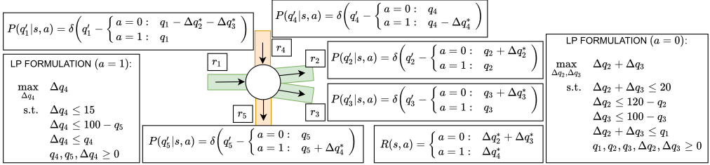
Example 1 (SIMPLE TRAFFIC MANAGEMENT). Figure 1 shows a road configuration where an Eastbound road (r1) intersects a Southbound road (r4). r1 diverges into r2 and r3 after the intersection, and r4 transitions to r5. Each road is one-way, and the state of the environment consists of traffic volumes on the roads, i.e. s = (q1, q2, q3, q4, q5). For simplicity, we assume cars do not leave r2, r3 and r5. The controller needs to decide which traffic approach to give a green light: r1 (a = 0) or r4 (a = 1). A positive reward is received for each vehicle transitioning through the intersection. The max capacities of roads r1, r2, r3, r4 and r5 are 100, 120, 100, 100 and 100 respectively. The max number of cars leaving r1 and r4 are capped at 20 and 15, respectively.

Notice that the ∆q∗ i terms in the transition equations (Figure 1) are the argmax solutions of the LP transition. Since the state transitions depend on the argmax of the LP, we have to symbolically obtain closed-form optimal solutions of the LP to provide an exact closed-form solution to the overall MDP. Hence, as our primary technical contribution in this work, we develop a multivariate symbolic argmax operator by breaking it into respective arg and max operations and showing that each can be computed in closed-form.

1 For purposes of concise exposition and explanation of the optimal value function and policy, this DC-MDP example uses continuous states and deterministic transitions; the empirical results will later discuss a range of DC-MDPs with stochastic transitions.

After preliminaries in Section 2, we first describe a univariate arg max operation in Section 3, followed by the extension to the multivariate case. The argmax operation facilitates a novel and exact closed-form SDP approach that we evaluate in Section 4 on problems from the Operations Research domain: SIMPLE TRAFFIC MANAGEMENT, RESERVOIR MANAGEMENT and BANDWIDTH OPTIMIZATION. We also compare our SDP approach with a discretized approximation showing that the SDP approach is more efficient and scalable without the error inherently induced by discretization.

2 Discrete and Continuous State MDPs

In a DC-MDP, vectors of variables (⃗b, ⃗x) = (b1, . . . , bn, x1, . . . , xm) represent a state. Each state variable bi (1 ≤ i ≤ n) is boolean s.t. bi ∈{0, 1} and each xj (1 ≤ j ≤ m) is continuous s.t. xj ∈[Lj,Uj] for Lj, Uj ∈ R. We also assume a finite set of actions A = {a1, . . . , a|A|}.

We define a DC-MDP by the following: (1) a transition model P(⃗b′ , ⃗x′ |⃗b, ⃗x, a) which specifies the probability of the next state (⃗b′ , ⃗x′ ) conditioned on the current state and action a; (2) a reward function R(⃗b, ⃗x, a) which specifies the immediate reward obtained by taking action a in state (⃗b, ⃗x); and (3) a discount factor γ, 0 ≤ γ ≤ 1. A policy π specifies the action π(⃗b, ⃗x) to take in each state (⃗b, ⃗x). Then, our goal is to find an optimal sequence of horizon-dependent policies Π∗ = (π∗,1 , . . . , π∗,H ) that maximizes V Π∗ (s0), the expected sum of discounted rewards over a horizon h; H ≥ 0:

Here rh is the reward obtained at horizon h while following Π∗ , and we assume a starting state s0 =(⃗b0, ⃗x0) at h = 0.

DC-MDPs as defined above are naturally factored in terms of state variables (⃗b, ⃗x) [Boutilier et al., 1999]; as such a transition structure can be exploited in the form of a dynamic Bayes net (DBN) [Dean and Kanazawa, 1989] where the individual conditional probabilities P(b′i| · · · , a) and P(x′j| · · · , a) condition on a subset of the current and next state variables. We disallow synchronic arcs (variables conditioning on each other in the same time step) within the binary ⃗b and continuous variables ⃗x, but we allow synchronic arcs from ⃗b to ⃗x (note: these conditions enforce the directed acyclic graph requirements of DBNs). We write the joint transition model as

where P(b′i|⃗b, ⃗x, a) may condition on a subset of ⃗b and ⃗x, and P (x′j |⃗b,⃗b′ , ⃗x, a) may condition on a subset of ⃗b,⃗b′ and ⃗x.

We refer to the conditional probabilities P(b′i|⃗b, ⃗x, a) for binary variables bi (1 ≤ i ≤ n) as conditional probability functions (CPFs) - not tabular enumerations because these functions can condition on both discrete and continuous states. For continuous variables xj (1 ≤ j ≤ m), we represent the CPFs P(x′j|⃗b, ⃗ b′ , ⃗x, a) as piecewise linear equations (PLEs) with three properties: (1) PLEs can only condition on the action, current state, and previous state variables; (2) PLEs are deterministic meaning that to be represented by probabilities, they must be encoded using Dirac δ[·] functions; and (3) PLEs are piecewise linear, where the piecewise conditions may be arbitrary logical combinations of ⃗b, ⃗b′ and linear inequalities over ⃗x. Example PLEs are in Figure 1 where the use of the δ[·] function ensures that this is a conditional probability function that integrates to 1 over x′j . PLEs allow modeling of continuous variable transitions as a mixture of δ functions used in continuous state MDP solutions [Meuleau et al., 2009].

2.1 Dynamic Programming Solution

A continuous state generalization of value iteration [Bellman, 1957] is a dynamic programming algorithm for computing the optimal value function V Π∗ in Eq.1. It proceeds by constructing a series of h-stage-to-go value functions V h (⃗b, ⃗x). Specifically, initializing V 0 (⃗b, ⃗x) (e.g., to V 0 (⃗b, ⃗x) = 0) we repeatedly compute the following for h ∈ {0, . . . , H - 1}:

2.2 Linear Program (LP) Transitions

In this paper, we consider DC-MDPs with LP transitions. In this set of problems, the state transition function over continuous state variables and the reward function depend on a pdimensional intermediate vector ⃗y∗ , that is, P(⃗ x′ |⃗b, ⃗ b′ , ⃗x, a, ⃗y∗ ) and R(⃗b, ⃗x, a, ⃗y∗ ); whereas the transition over binary state variables remains as in Eq.2. Here, ⃗y∗ is determined by the following LP given a fixed state and action ⃗b, ⃗x, a:

where Dy ∈ Rp is the domain of the continuous vector ⃗y; φi (1 ≤ i ≤ k) and f are respectively the linear constraints and the linear objective of the LP.

3 Symbolic Dynamic Programming

In this section, we review and extend the symbolic dynamic programming (SDP) framework of value iteration (VI) for DC-MDPs [Sanner et al., 2011] to accommodate LP transitions. Continuous action [Zamani et al., 2012; Zamani et al., 2013] extensions are straightforward but omitted for clarity.

3.1 Case Operators and SDP

In SDP, we assume that all symbolic functions can be represented in case form [Boutilier et al., 2001]:

Here φi are logical formulae defined over the state s = (⃗b, ⃗x) and the intermediate variable ⃗y from Eq.5, which can include arbitrary logical (∧, ∨, ¬) combinations of (1) boolean variables and (2) linear inequalities (≥,>,≤,<) over continuous variables. Each φi will be disjoint from the other φj (j ̸= i); however, φi may not exhaustively cover the entire domain, so f may be undefined for some variable assignments. In this work, we assume the fi are also linear in the continuous variables. Furthermore, we require f to be continuous (including no discontinuities at partition boundaries); case operations will then preserve this property.

Unary operations such as scalar multiplication c·f (c ∈ R) or negation -f on case statements are simply applied to each fi (1 ≤ i ≤ k). To perform a binary operation on two case statements, we take the cross-product of the logical partitions of each case statement and perform the operation on the resulting paired partitions. Letting each φi and ψj denote generic first-order formulae, we can perform the "cross-sum" ⊕ of two (unnamed) cases in the following manner:

Likewise, we perform ⊖ and ⊗ by, respectively, subtracting or multiplying partition values to obtain the result. Some partitions resulting from case operators may be infeasible and removed.

Next, we define symbolic case maximization whose result is still piecewise linear:

Another important operation is symbolic substitution. The operation takes a set σ of variables and their substitutions, e.g., σ = {x′1 /(x1 + x2), x′2 /(x1 - x2)} where the LHS of / represents the substitution variable and the RHS of / is the expression that should be substituted in. Then, we write the substitution of a non-case function fi with σ as fiσ. We can also substitute into case partitions φj by applying σ to each inequality operand. Then, we can define the substitution operation for case statements in general:

With the insight that integration over PLEs reduces to symbolic substitution [Sanner et al., 2011], SDP simply executes value iteration in Eqs. 3 and 4 using the DC-MDP definition defined previously and the case operators defined above to yield a closed-form, exact symbolic derivation of the value function [Sanner et al., 2011].

3.2 Multivariate Symbolic max Operator

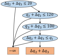
Before we proceed to extend SDP to DC-MDPs with LP transitions, we first have to understand how to represent and manipulate an LP in the symbolic case notation. To this end, note that an LP (Eq. 5) has a natural case structure and can be represented even more compactly in XADD form [Sanner et al., 2011] shown in Figure 2: every leaf shows a value fi and every path from root to leaf is uniquely associated with one partition φi (a conjunction of decisions) and the value fi. A solid line from a decision node to another node indicates the true branch of the parent node, while a dotted line shows the false branch. Each decision node corresponds to a constraint of the LP, and false branches lead to the -∞ node. This is an intuitive way to specify LP infeasibility as we are solving a maximization problem. We denote the LP as f(⃗x,⃗b, ⃗y).

Symbolically solving an LP amounts to symbolically maximizing out continuous variables from the case statement. Thus, we adopt the approach in [Zamani et al., 2012] to make three observations: (1) multivariate maximization can be decomposed into a series of univariate maximizations; (2) to maximize a case statement w.r.t. a variable yl (1 ≤ l ≤ p), we need to perform a symbolic maxyl on each case partition then combine results via casemax; (3) a partition φi defines lower (LBi) and/or upper (UBi) bounds over yl. Since fi is linear, the max of fi has to occur at one of the bounds. I.e.,

where φi,ind includes LBi ≤ UBi and decisions in φi that are independent of yl. σlb i = {yl/LBi} and σub i = {yl/UBi} represent substitution of the lower and upper bounds to yl in fi, respectively. Note that LBi and UBi are also symbolic case functions (see the example in the following section).

3.3 Multivariate Symbolic argmax Operator

We now introduce the novel symbolic arg max operation that will allow us to analytically solve for the solution of our LP transitions in Eq.5, substitute this symbolic LP solution to reduce our transitions to a standard DC-MDP, and then apply the known SDP solution for this reduced DC-MDP.

For each (φi, fi), either yl = LBi or UBi will output the max in Eq.7. So, we annotate fi accordingly to keep track of which yl value has resulted in the max for the particular logical partition. Let f(⃗x,⃗b, ⃗y-l) = maxyl f(⃗x,⃗b, ⃗y). If we assume - for the sake of simplicity - the values of casemax(fiσlb i , fiσub i ) are different for all i (1 ≤ i ≤ k)2 , then every function value of f(⃗x,⃗b, ⃗y-l) can be uniquely traced back to an annotated yl as follows:

Here, each partition ψj (1 ≤ j ≤ k′ ) has an associated function value f(j,-yl) and annotation oj .

The trick is to split argmax into arg and max. Once we obtain f(⃗x,⃗b, ⃗y-l) from max, we perform arg on it to retrieve the annotations and to build a symbolic case statement representing argmaxyl f(⃗x,⃗b, ⃗y) as in Eq.9.

2 When the two arguments are the same for some i, we can have multiple optimal solutions. As often done by off-the-shelf LP solvers, we simply select one optimal solution in this case.

The arg operation removes f(j,-yl) from ψj and leaves oj only. Note that oj can be a case function, in which case the partitions in oj are combined with ψj and simplified.

For the multivariate argmax, let's assume we maximize y1, . . . , yp in this order, namely max⃗ y f(⃗x,⃗b, ⃗y) = maxyp · · · maxy1 f(⃗x,⃗b, ⃗y). Then, we repeat the following steps p times:

1. Compute the innermost maximization f(⃗x,⃗b, ⃗y-(1:l)) = maxyl f(⃗x,⃗b, ⃗y-(1:l-1));
2. Perform arg operation on f(⃗x,⃗b, ⃗y-(1:l)) to get y∗ l .

This way, we obtain y∗ l for all l = 1, . . . , p in case form. Note that y∗ l will still contain 'outer' variables yl′ (l + 1 ≤ l′ ≤ p) in its case statement. However, in order to get a closedform symbolic solution to MDPs with LP transitions, we need to be able to express each y∗ l only with⃗b, ⃗ b′ , ⃗x.

Removing outer variables from the case statement of y∗ l involves repeated substitution of y∗ l′ . Observe that y∗ p contains only ⃗b, ⃗ b′ , ⃗x, while y∗ p-1 additionally has yp. Therefore by substituting y∗ p into y∗ p-1 , it now contains ⃗b, ⃗ b′ , ⃗x only. For y∗ p-2 , we need to substitute both y∗ p and the modified y∗ p-1 . This process should be repeated for all yl (1 ≤ l ≤ p - 1).

However, we cannot substitute y∗ l+1 into y∗ l via the symbolic substitution since y∗ l+1 is also a case statement. Instead, we merge two case statements as described in Example 2.

Example 2. Define g(x, y) and y = h(x) as follows:

When we substitute y = h(x) into g(x, y), we get

So, we take the cross-product of the logical partitions and substitute an appropriate value of y into g(x, y).

We summarize in four major steps how to get a closed-form argmax solution to an LP using the a = 0 case in Example 1. We denote the LP in case form as f(q1, q2, q3, ∆q2, ∆q3).

1. Univariate maximization with annotation. In Figure 2, the feasible partition consists of {(∆q2 + ∆q3 ≤ 20) ∧ (q2 + ∆q2 ≤ 120) ∧ (q3 +∆q3 ≤ 100) ∧ (∆q2 +∆q3 ≤ q1)}. Call this partition φi, then we have φi : fi = ∆q2 +∆q3 and φj : -∞ (j ̸= i). When we maximize out ∆q2, decisions in φi and a domain bound ∆q2 ∈ [0, 20] define UB and LB of ∆q2. For example, UB = casemin(20, 20 - ∆q3, 120 - q2, q1-∆q3), which becomes the following case statement:

The maximum of fi occurs either at ∆q2 = UB or LB. Hence, we take casemax to determine the max, that is,

Then, we incorporate independent decisions: LB ≤ UB and q3 +∆q3 ≤ 100. We refer readers to [Zamani et al., 2012] for the step-by-step walk-through. The difference is that we annotate values with either LB or UB.

1. Annotation preserving casemax. Once continuous max is done, we take casemax and obtain f(q1, q2, q3,∆q3). This step preserves the annotations from Step 1.
2. Application of arg operator. We then compute ∆q∗ 2 = arg∆q2 f(q1, q2, q3,∆q3) (Eq.9).

We repeat Step 1-3 on f(q1, q2, q3,∆q3) to maximize over ∆q3, producing f(q1, q2, q3). Then, ∆q∗ 3 is a case function of q1, q2, q3, while ∆q∗ 2 is a case function of q1, q2, q3,∆q3.

1. Case substitutions. Finally, we substitute the case statement ∆q∗ 3 into ∆q∗ 2. Both are now functions of q1, q2, q3 and are used in defining the state transition function.

3.4 SDP with LP Transitions

Having introduced the symbolic argmax operator, we can symbolically solve Eq.5, resulting in a case function u(⃗b, ⃗x, a) in Eq.10. This step only has to occur once. Subsequently, we define a symbolic substitution σ⃗ y∗ to substitute the solution into the transition and reward functions (as in Eq.11-13).

Overall, we have reduced a DC-MDP with LP transitions to a standard DC-MDP, which can be solved in closed-form by leveraging its SDP solution (Section 3.1).

4 Empirical Results

We now apply our methodology for exact SDP with LP transitions to SIMPLE TRAFFIC MANAGEMENT, RESERVOIR MANAGEMENT, and BANDWIDTH OPTIMIZATION. 3

We also compare to approaches that discretize the state space of the DC-MDP as discussed in Section 1. While LP transitions may suggest some form of mixed integer linear program (MILP) solution, we note that existing MILP-based solutions for finite horizon DC-MDPs (with no LP transitions) [A. Raghavan et al., 2017] provide no error guarantees and only solve for a known starting state, whereas our SDP approach provides an exact value function for all states.

SIMPLE TRAFFIC MANAGEMENT. Figure 3 (left) shows the symbolic and approximate value function, V 13 (q1, q4) for H = 13. We observe that locations in the state space where all available vehicles in roads r1 and r4 can be accommodated within destination lanes show a much higher slope in the value function. These are regions where q1 and q4 are closer to their lower domain limits. As q1 reaches a threshold value, all available spaces in q2 and q3 have filled, and there is no consequent gain in value with increase in q1. A similar observation can also be made for q4. The value function maxes out when all destination lanes have reached capacity.

3 Implementations can be found at https://github.com/ jihwan-jeong/xadd-inference/. Additional information regarding the empirical evaluations can also be found in Appendix.

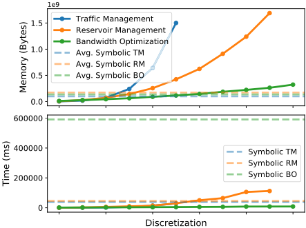
The approximate value function can only be obtained for a maximum discretization of 14 before it's no longer feasible to solve for a finer granularity due to a memory explosion as evident in Figure 4. This shows the accuracy and computational limitations of approximate discretization solutions.

RESERVOIR MANAGEMENT. In a Reservoir management problem [Mahootchi, 2009; Yeh, 1985], we examine a 2reservoir system with one upstream reservoir (r1) having no electricity generation facility and one downstream reservoir (r2) with a hydroelectric power generator. The decision is whether to allow or block the flow of water between the two reservoirs. Water is always discharged from r2 within its operating bounds to produce maximum electricity according to an LP optimization. Water evaporates from a reservoir with the amount proportional to the water level li. When the water level is close to its lower limit, we allow a small amount of water to flow into a reservoir to make the LP in Eq.14 feasible. Finally, the stochastic rainfall is described in Eq.15.

The state vector consists of two continuous variables and one binary variable, i.e. s = (l1, l2, r). The associated transition LP and the resulting state transitions are as follows:

where the water flow is blocked when a = 0, and allowed within a limit when a = 1. q∗ 1 , q∗ 2 are argmax of Eq.14, and we can see that q∗ 1 , q∗ 2 are case functions of l1, l2, r and a.

Figure 3 (middle) shows the value function for the RESERVOIR MANAGEMENT problem for H = 4, V 4 (l1, l2, r = False). We can see that regions where q1 and q4 are close to their domain upper limits correspond to areas with the highest values. The symbolic and the approximate solution have similar surface contours but approximation error still creeps in, especially in regions where l1 is high and l2 is low.

BANDWIDTH OPTIMIZATION. In a bandwidth optimization problem [Adler et al., 2011], a service provider is given a network traffic demand from users, and the company needs to purchase bandwidths from ISPs (Internet service providers). In each time period, the company subscribes to a different set of links (with differing costs) offered by different ISPs to meet the current demand and residual demand from previous time steps while minimizing operating costs.

Now, consider a simple network with 5 links (L = {o1, o2, 12, 1e, 2e}) and 3 paths (o → 1 → e, o → 1 → 2 → e, o → 2 → e) from the origin (o) to the edge server (e). The company has 7 buying options (|A| = 7), each of which corresponds to purchasing a different combination of paths. We firstly define the associated max flow problem:

where xij is the max flow on link ij and Kij is its capacity. Eq.17 enforces the balance in flow at every node. Also, given a buying option, bij = 1 for the links on the paths. Otherwise, bij = 0, thereby restricting xij to 0.

We assume the following pricing policy: the provider pays (i) mij for purchasing the bandwidth on link ij and (ii) a fee as per the actual traffic routed on the link (c·xij with unit cost c). Then the states, actions and rewards are defined as below:

• State s = (d, l) where d ∈ R+ is the remaining demand and l ∈ {0, 1} (low, high) is the level of new demand.
• Action {a1, . . . , a7}.
• Reward: R(d, l, a) = r · xd - p · (d - xd) - c · xd - ∑i,j∈N mij ·bij . Here, xd = min(d, x∗o1 +x∗o2 ) is the actual routed traffic to meet the demand d. r and p are the unit revenue for the traffic delivered and the unit penalty for unmet demands, respectively.

The state transition is defined as the following, where dnew = 2500 when l = high and dnew = 1200 otherwise:

Time and Space. Figure 4 shows the time and space complexity of approximate solutions along with that of the symbolic solutions. As before, we see an exponential blowup for the approximate discretized solution as the discretization granularity increases. We also note that as the number of state variables vary between problems, the discretization-based approach suffers from the curse of dimensionality with respect to memory requirements, while in stark contrast, the SDP solution size is independent of the number of state variables.

5 RelatedWork and Concluding Remarks

Building on a line of continuous state MDP solutions [Boyan and Littman, 2001; Feng et al., 2004; Li and Littman, 2005; Sanner et al., 2011], we proposed a novel symbolic dynamic programming (SDP) method for exactly solving DC-MDPs with LP transitions. Specifically, we extended the symbolic max operator [Zamani et al., 2012] to an argmax operator via annotation augmentations to the case notation and its operations. Overall, this work provides the first exact solution method for DC-MDPs with LP transitions, and hence opens up a new class of challenging MDPs for research exploration.

For future work, one could leverage initial state focused techniques [Meuleau et al., 2009; Vianna et al., 2015] to reduce solution scope and size. Recent advances from Weighted Model Integration (WMI) [Kolb et al., 2018] may speed up computation of the symbolic max and argmax. Finally, methods for approximately bounding optimal value function structure [St-Aubin et al., 2000; Vianna et al., 2013] or further afield [Remi Munos, 2002; Kveton et al., 2006; Marecki et al., 2007] may improve scalability.