
A Fast Algorithm for Optimally Finding Partially Disjoint Shortest Paths
Proceedings of the Twenty-Seventh International Joint Conference on Artificial Intelligence. Main track. Pages 1456-1462.
https://doi.org/10.24963/ijcai.2018/202
Keywords
- Heuristic Search and Game Playing: Combinatorial Search and Optimisation
- Multidisciplinary Topics and Applications: AI and the Web
- Multidisciplinary Topics and Applications: Databases
Abstract
The classical disjoint shortest path problem has recently recalled
interests from researchers in the network planning and optimization
community. However, the requirement of the shortest paths being completely
vertex or edge disjoint might be too restrictive and demands much
more resources in a network. Partially disjoint shortest paths, in
which a bounded number of shared vertices or edges is allowed, balance
between degree of disjointness and occupied network resources.
In this paper, we consider the problem of finding k
shortest paths which are edge disjoint but partially vertex disjoint.
For a pair of distinct vertices in a network graph, the problem aims
to optimally find k edge disjoint shortest paths among which
at most a bounded number of vertices are shared by at least two paths. In particular,
we present novel techniques for exactly solving the problem
with a runtime that significantly improves
the current best result. The
proposed algorithm is also validated by computer experiments on both
synthetic and real networks which demonstrate its superior efficiency
of up to three orders of magnitude faster than the state of the art.
- Email-Enron 36,692 183,831 20.76 Email-EuAll 265,214 420,045 35.04 p2p-Gnut.05 8,846 31,839 2.55 p2p-Gnut.06 8,717 31,525 2.94 p2p-Gnut.08 6,301 20,777 1.92 Networks #Nodes #Edges EA (s) p2p-Gnut.09 8,114 26,013 2.40 p2p-Gnut.24 26,518 65,369 6.02 p2p-Gnut.25 22,687 54,705 5.13 p2p-Gnut.30 36,682 88,328 8.44 p2p-Gnut.31 62,586 147,892 13.40
- [Ahuja et al., 1993] Ravindra K Ahuja, Thomas L Magnanti, and James B Orlin. Network flows: theory, algorithms, and applications. 1993.
- [Akiba et al., 2015] Takuya Akiba, Takanori Hayashi, No- zomi Nori, Yoichi Iwata, and Yuichi Yoshida. Efficient top-k shortest-path distance queries on large networks by pruned landmark labeling. In AAAI, volume 15, pages 25- 30, 2015.
- [Andrews et al., 2005] Matthew Andrews, Julia Chuzhoy, Sanjeev Khanna, and Lisa Zhang. Hardness of the undi- rected edge-disjoint paths problem with congestion. In Foundations of Computer Science, 2005. FOCS 2005. 46th Annual IEEE Symposium on, pages 226-241. IEEE, 2005.
- [Andrews, 2010] Matthew Andrews. Approximation algo- rithms for the edge-disjoint paths problem via raecke decompositions. In Foundations of Computer Science (FOCS), 2010 51st Annual IEEE Symposium on, pages 277-286. IEEE, 2010.
- [Chekuri and Ene, 2013] Chandra Chekuri and Alina Ene. Poly-logarithmic approximation for maximum node dis- joint paths with constant congestion. In Proceedings of the twenty-fourth annual ACM-SIAM symposium on Discrete algorithms, pages 326-341. Society for Industrial and Ap- plied Mathematics, 2013.
- [Chekuri et al., 2005] Chandra Chekuri, Sanjeev Khanna, and F Bruce Shepherd. Multicommodity flow, well-linked terminals, and routing problems. In Proceedings of the thirty-seventh annual ACM symposium on Theory of com- puting, pages 183-192. ACM, 2005.
- [Chuzhoy, 2016] Julia Chuzhoy. Routing in undirected graphs with constant congestion. SIAM Journal on Com- puting, 45(4):1490-1532, 2016.
- [Cormen, 2009] Thomas H Cormen. Introduction to algo- rithms. MIT press, 2009.
- [Garey and Johnson, 2002] Michael R Garey and David S Johnson. Computers and intractability, volume 29. wh freeman New York, 2002.
- [Guo et al., 2015] Longkun Guo, Kewen Liao, Hong Shen, and Peng Li. Brief announcement: Efficient approxima- tion algorithms for computing k disjoint restricted short- est paths. In Proceedings of the 27th ACM symposium on Parallelism in Algorithms and Architectures, pages 62-64. ACM, 2015.
- [Hansen and Abdoulahi, 2016] Eric A Hansen and Ibrahim Abdoulahi. General error bounds in heuristic search al- gorithms for stochastic shortest path problems. In AAAI, pages 3130-3137, 2016.
- [Hassin, 1992] Refael Hassin. Approximation schemes for the restricted shortest path problem. Mathematics of Op- erations research, 17(1):36-42, 1992.
- [Imamichi et al., 2016] Takashi Imamichi, Takayuki Os- ogami, and Rudy Raymond. Truncating shortest path search for efficient map-matching. In IJCAI, pages 589- 595, 2016. IJCAI
- [Joksch, 1966] Hans C Joksch. The shortest route problem with constraints. Journal of Mathematical analysis and applications, 14(2):191-197, 1966.
- [Kurose and Ross, 2009] James F Kurose and Keith W Ross. Computer networking: a top-down approach, volume 4. Addison Wesley Boston, USA, 2009.
- [Lorenz and Raz, 2001] Dean H Lorenz and Danny Raz. A simple efficient approximation scheme for the restricted shortest path problem. Operations Research Letters, 28(5):213-219, 2001.
- [Orda and Sprintson, 2004] Ariel Orda and Alexander Sprintson. Efficient algorithms for computing disjoint qos paths. In INFOCOM 2004. Twenty-third AnnualJoint Conference of the IEEE Computer and Communications Societies, volume 1. IEEE, 2004.
- [Raghavan and Tompson, 1987] Prabhakar Raghavan and Clark D Tompson. Randomized rounding: a technique for provably good algorithms and algorithmic proofs. Combi- natorica, 7(4):365-374, 1987.
- [Seymour and Kar, 2013] Zachary Seymour and Dulal Kar. Finding partially link-disjoint paths in wireless sensor net- works. In Wireless Conference (EW), Proceedings of the 2013 19th European, pages 1-6. VDE, 2013.
- [Suurballe and Tarjan, 1984] JW Suurballe and RE Tarjan. A quick method for finding shortest pairs of disjoint paths. Networks, 14(2):325-336, 1984.
- [Suurballe, 1974] JW Suurballe. Disjoint paths in a network. Networks, 4(2):125-145, 1974.
- [Yallouz et al., 2016] Jose Yallouz, Ori Rottenstreich, Peter Babarczi, Avi Mendelson, and Ariel Orda. Optimal link- disjoint node-"somewhat disjoint" paths. In Network Pro- tocols (ICNP), 2016 IEEE 24th International Conference on, pages 1-10. IEEE, 2016.
References were extracted automatically from the PDF and may contain errors.
Full text extracted automatically from the PDF; figures, tables and equations may differ. The PDF is the version of record.
1 Introduction
Several shortest path problems [Akiba et al., 2015; Hansen and Abdoulahi, 2016; Imamichi et al., 2016] have recently witnessed renewed interests in AI community. Solutions to these problems are largely heuristic-based. In network planning and optimization, the classical disjoint shortest path problem, especially the problem of finding partially disjoint shortest paths, has also started with a heuristic method [Seymour and Kar, 2013] and only recently seen guaranteed optimal solutions [Yallouz et al., 2016]. However, the state-ofart optimal solutions are far from being efficient and scalable, limiting their practicability. In this paper, we investigate a fast solution to the following problem of finding k edge-disjoint shortest paths with a bounded number of common vertices:
∗These two authors share equal contribution.
Definition 1. (The δ-vertex k edge-disjoint shortest path problem, δV-kEDSP): For a directed graph or network G = (V, E) with a source vertex s ∈ V and a destination t ∈ V , a weight function w : E → Z +, a given nonnegative integer δ ∈ Z, δV-kEDSP aims to compute k edge-disjoint paths P1, P2, · · · , Pk in G, such that ∑i=1, ··· , k w (Pi) attains the minimum while among them there are at most δ vertices (besides s and t) shared by at least two paths.
Intuitively, the above definition constrains edge-disjoint shortest paths intersecting each other with the number of intersection (node) points upper bounded by δ. Compared with the other stricter vertex-disjoint shortest paths problem, δVkEDSP potentially finds a set of paths with a shorter average length. For the problem when k = 2, we propose a fast optimal (or namely exact) algorithm to δV-2EDSP, as we can already envision that the general δV-kEDSP requires much more algorithmic machinery. Note that throughout the paper we use terms "shortest" and "minimum weight", and also "exact algorithm" and "optimal algorithm", interchangeably.
1.1 RelatedWork
To the best of our knowledge, the δV-kEDSP problem was first studied in [Yallouz et al., 2016] for k = 2, where it was optimally solved within a time complexity O (mn2 +n3 logn). Although the study over δV-kEDSP is emerging, the case of δ = 0 has already attracted intensive research from mathematicians and computer scientists starting from early 70s. When δ = 0, δV-kEDSP becomes the complete vertex-disjoint (edge-disjoint) shortest st-path problem, namely the min-sum vertex-disjoint path problem, which can be simply solved with a simple max flow. It was also shown by Suurballe that the problem, for any fixed integer k > 0, admits an optimal algorithm with a runtime O(n2 log n) [Suurballe, 1974]. Later in [Suurballe and Tarjan, 1984], this runtime was improved to O (m log(1+m/n) n).
Another important variant of δV-kEDSP is the NodeDisjoint Path with Congestion (NDPwC) problem. The problem is to maximize the number of paths to respectively connect k given pairs of vertices s1t1, . . . , siti, . . . , sktk, such that each vertex appears on at most γ paths for a given positive integer γ that is known as congestion factor [Chekuri et al., 2005; Chekuri and Ene, 2013]. The existing methods mostly modeled and relaxed the NDPwC problem as a natural multicommodity flow problem via linear programming. Chekuri et al [Chekuri et al., 2005] used the multicommodity flow LP-relaxation to obtain an O (log2 k log n) approximation with congestion γ = 4 for NDPwC in planar graph. Then, Chekuri and Ene [Chekuri and Ene, 2013] gave a polynomial time algorithmwhich routes Ω( OPT poly log k ) pairs with O(1) congestion in undirected graphs, where OPT is the value of an optimal fractional solution to a natural multicommodity flow relaxation. For the edge-disjoint case, the edge-disjoint path with congestion (EDPwC) problem is also to maximize the number of disjoint paths respectively connecting the given pairs of vertices, such that each edge appears on at most γ paths. For the first time addressing EDPwC, Raghavan and Thompson [Raghavan and Tompson, 1987] gave a constant factor approximation with congestion γ relaxed to Ω(log n/ log log n) by using randomized rounding technique. Later, Andrew presented a randomized (O(log61 n), O((log log n)6 ))-approximation algorithm for EDPwC in [Andrews, 2010]. Note that for inapproximability, Andrews et al. [Andrews et al., 2005] have also shown that for any congestion γ = O( log log n log log log n ), there is no log 1-ϵ γ+1 n-approximation algorithm for EDPwC unless NP ⊆ ZPTIME(npoly log n ), so their poly-logarithmic bifactor ratio is nearly the best possible. For better congestion guarantee but fewer paths between pairs of vertices, Chuzhoy in [Chuzhoy, 2016] recently gave an efficient randomized algorithm, which routes Ω( OPT log22.5 k log log k ) demand pairs with congestion of at most 14.
Our techniques for solving δV-kEDSP involve at the last step a transformation to the restricted shortest path (RSP) problem that is known NP-complete in [Garey and Johnson, 2002]. To the best of our knowledge, Joksch [Joksch, 1966] was the first to formally solve RSP by presenting a pseudo-polynomial time algorithm using dynamic programming. Although we adopt this pseudo-polynomial algorithm for RSP to form our polynomial time solution (this works because in our case δ ≤ n), it is worthwhile to mention other related approximations: Hassin gave another pseudo-polynomial algorithm with runtime O(mOPT) for OPT being the weight of an optimal solution, and then consequently gave an FPTAS with time O (m ( n2 ϵ ) log ( nϵ )) [Hassin, 1992]; While Lorena and Raz [Lorenz and Raz, 2001] proposed another FPTAS with a further improved runtime O (mn (log log n + 1ϵ )), for any fixed real number ϵ > 0. Recently, the research interest is also on the k-edge (vertex) disjoint restricted shortest path (kRSP) problem which combines RSP and disjoint paths [Orda and Sprintson, 2004; Guo et al., 2015].
1.2 Our Results
In this paper, we propose an exact algorithm for δV-2EDSP with a runtime O(δm+n log n), which significantly improves the runtime O(mn2 + n3 log n) of the previous best solution [Yallouz et al., 2016]. Our algorithm is based on the main observation that, if δV-2EDSP is feasible then there must exist a special optimal solution, what we called a spiral optimal solution. The algorithm progresses with the idea of path augmentation. It first computes a shortest st-path, then this path gets augmented to a pair of spiral st-paths via our specially constructed residual graph with an extra cost function to capture the number of shared vertices. Moreover, we show that if δV-2EDSP is feasible, then there must exist a spiral optimal solution whose shared vertices are all on the shortest st-path. With techniques from graph theory and network flow theory, we prove that our algorithm produces an optimal solution to δV-2EDSP. The proposed algorithm has the potential to extend to δV-kEDSP for general k, but we omit this discussion here due to space limit. We also run experiments on both synthetic and real networks to validate the practical performance of our algorithm against other baselines. Experimental results show an up to three orders of magnitude runtime reduction - matching our theoretical runtime analysis.
2 Exact Algorithms for δV-2EDSP
In this section, we first focus on an important property of δV2EDSP: there must exist a special optimal solution called spiral optimal solution if an instance of δV-2EDSP is feasible. Then we give an algorithm to compute such a spiral optimal solution, which equivalently solves δV-2EDSP.
2.1 Spiral Optimal Solutions to δV-2EDSP
We denote a network by a digraph G = (V, E), where V and E are respectively the sets of vertices and edges. Assume that n = |V | and m = |E|. Given an st-path P and two vertices u, v ∈ P, we denote by P(u, v) the subpath of P from u to v, and say u ≺P v if and only if v ̸= u appears on P(u, t), i.e. v ∈ P(u, t). For two paths P1 and P2, we say P1(u, v) is a maximal segment within P1 ∩P2 iff (1) P1(u, v) ⊆ P1 ∩P2 and (2) there exists in P1 ∩P2 no other segment that contains P1(u, v), that is, there exists no Pi(x, y) ⊆ P1 ∩ P2, i ∈ {1, 2}, such that Pi(x, y) ⊃ P1(u, v) holds.
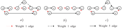
Our algorithm will actually compute a special optimal solution called a spiral optimal solution, which is formally as follows (An example comparing a spiral optimal solution vs a non-spiral optimal solution is as depicted in Figure 1):
Definition 2. Let P ∗ be a shortest st-path in G. Then an optimal solution to δV-2EDSP, say P = {P ∗ 1 , P ∗ 2 }, is a spiral optimal solution if the following two conditions both hold: (1) For any u, v ∈ P ∗ ∩P ∗ i , i ∈ {1, 2}, u ≺P∗ v iff u ≺P∗ i v; (2) Let Si = P ∗ ∩P ∗ i , i ∈ {1, 2}, be the set of maximal segments at which P ∗ intersects with P ∗ i . Then for any segj, segj ′ ∈ Si, i ∈ {1, 2}, if segj ≺P∗ i segj ′ then there must exist seg ∈ S3-i, such that segj ≺P∗ seg ≺P∗ segj ′ holds on P ∗ .
Note that P ∗ 1 and P ∗ 2 in the above definition must be edgedisjoint and hence can only share common vertices.
We say vj, vj ′ ∈ P ∗ ∩P ∗ i , i ∈ {1, 2} are properly ordered, if vj, vj ′ satisfy Condition 1; Otherwise, say vj ≺ vj ′ on P ∗ while vj ′ ≺ vj on P ∗ i , vj and vj ′ is antiordered. Note that there may exist P ∗ i ∈ P, i ∈ {1, 2}, such that P ∗ = P ∗ i .
The key idea of our algorithm is inspired by the Simplex method of solving linear programs, in which a special optimal solution called basic optimal solution, rather than any optimal solution, is computed. So similar to the correctness proof of the Simplex method, we need first to show it suffices to compute a spiral optimal solution to solve δV-2EDSP, as given in the following theorem:
Theorem 3. If an instance of δV-2EDSP is feasible, then it must have spiral optimal solutions.
Proof. For Condition 1 of Definition 2, we show that if an instance of δV-2EDSP is feasible, then an optimal solution can be constructed satisfying the condition. Assume {P ∗ 1 , P ∗ 2 } is an optimal solution of δV-2EDSP, for which there exist vj, vj ′ ∈ P ∗ ∩ P ∗ i , i ∈ {1, 2}, such that vj ≺ vj ′ on P ∗ but vj ′ ≺ vj on P ∗ i . Then we can construct a pair of disjoint path P1 and P2 of which the number of antiordered vertex pairs decreases at least one comparing to {P ∗ 1 , P ∗ 2 }. Consequently, an optimal solution without any antiordered vertex pair can be constructed by repeatedly decreasing the number of antiordered vertex pairs.
It remains to give the construction of P1 and P2. Without loss of generality, we assume that vj ′ is the vertex closest to t in all antiordered vertex pairs. Let u, which belongs to Pi ∪ P3-i, be the first vertex after vj ′ . We will construct P1 and P2 for both two cases that u ∈ P ∗ i or u ∈ P ∗ 3-i :
(1) u ∈ P ∗ 3-i : Let w ∈ P ∗ 3-i ∩ P ∗ be the last vertex before vj. We will show that there exists a solution P1 and P2 whose weight is not larger than that of P ∗ 1 and P ∗ 2 , but with fewer antiordered vertex pairs. We need only to simply set P1 = P ∗ i (s, vj ′) ∪ P ∗ (vj ′ , u) ∪ P ∗ 3-i (u, t) and P2 = P ∗ 3-i (s, w) ∪ P ∗ (w, vj) ∪ P ∗ i (vj, t). Apparently, every properly ordered vertex pair in {P ∗ 1 , P ∗ 2 } remains so while the antiordered vertex pair {vj , vj ′ } becomes also properly ordered in P1 and P2. That is, the number of antiordered vertex pairs decreases at least one from {P ∗ 1 , P ∗ 2 } to {P1, P2}. It remains only to show the weight of {P1, P2} is not larger than {P ∗ 1 , P ∗ 2 }, which is to show w(P ∗ (vj ′ , u)∪P ∗ (w, vj)) ≤ w(P ∗ i (vj ′ , vj)∪P ∗ 3-i (w, u)). Suppose otherwise, i.e., w(P ∗ (vj ′ , u) ∪ P ∗ (w, vj)) > w(P ∗ i (vj ′ , vj), P ∗ 3-i (w, u)) ≥ w(P ∗ 3-i (w, u)). Then P = P ∗ (s, w)∪P ∗ 3-j (w, u)∪P ∗ (u, t) is an st-path with a smaller weight than P ∗ , contradicting with the optimality of P ∗ . Therefore, the two constructed paths P1 and P2 are with a weight that is not larger than {P ∗ 1 , P ∗ 2 }.
(2) u ∈ P ∗ i : We will construct a new path Pi, which is with a weight no larger than P ∗ i but at least one less antiordered vertex pair. For the task, we need only to simply set Pi = P ∗ i (s, vj ′) ∪ P ∗ (vj ′ , u) ∪ P ∗ i (u, t). Apparently, w(Pi) ≤ w(P ∗ i ), because w(P ∗ (vj ′ , u)) ≤ w(P ∗ i (vj ′ , vj)∪ P ∗ i (vj, u)) holds from the optimality of P ∗ . Besides, since vj /∈ Pi, Pi is with at least one less antiordered vertex pair than P ∗ i . Moreover, according to the construction of Pi, the path pair {Pi, P ∗ 3-i} shares only common vertices of the original {P ∗ i , P ∗ 3-i }, and hence {Pi, P ∗ 3-i } shares at most the same number of common vertices as {P ∗ i , P ∗ 3-i} which is bounded by δ.
For Condition 2, let {P ∗ 1 , P ∗ 2 } be an optimal solution to δV-2EDSP that already satisfies Condition 1. Then we show an optimal solution also satisfying Condition 2 can be constructed from {P ∗ 1 , P ∗ 2 }. Let segj and segj ′ be two segments in which all the interior vertices belong to S1 = {seg | seg ⊆ P ∗ 1 ∩ P ∗ }. Let u be the last vertex in segj and v be the first vertex in segj ′ . Assume that there exists no segment of S2 = {seg | seg ⊆ P ∗ 1 ∩P ∗ } that appears on P ∗ between segj and segj ′ . Then let P1 = P ∗ 1 (s, u)∪P ∗ (u, v)∪P ∗ 1 (v, t), which is P ∗ 1 excepting replacing P ∗ 1 (u, v), the subpaths of P ∗ 1 between segj and segj ′ , by P ∗ (u, v). Apparently, P ∗ (u, v) is with a weight no larger than P ∗ 1 (u, v), so w(P1) ≤ w(P ∗ 1 ). Moreover, segj and segj ′ are merged into one segment on P1. Besides, P1 and P ∗ 2 share only common vertices of P ∗ 1 and P ∗ 2 . Therefore, by repeating such operations, clearly such a {P ∗ 1 , P ∗ 2 } can eventually become a solution to δV-2EDSP satisfying both Condition 1 and Condition 2.
Note that, Condition 2 will not hold trivially without Condition 1. Because in that case we could not simply use P ∗ (u, v) to connect segj and segj ′ , as segj ′ ≺P∗ 1 segj ′ may hold. That is why we prove Condition 1 before Condition 2. Moreover, because P ∗ 1 and P ∗ 2 , as a spiral optimal solution to δV-2EDSP, are allowed to share δ common vertices, we have further observation on the relationship between their common vertices and P ∗ as below:
Lemma 4. If an instance of δV-2EDSP is feasible, there must exist a spiral optimal solution P ∗ 1 and P ∗ 2 wrt P ∗ , such that the common vertices of P ∗ 1 and P ∗ 2 are all on P ∗ , i.e. (V (P ∗ 1 ) ∩ V (P ∗ 2 )) ⊆ P ∗ .
Proof. Suppose otherwise, then there exists a common vertex of P ∗ 1 and P ∗ 2 that does not belong to P ∗ , say p ∈ P ∗ 1 ∩ P ∗ 2 that p /∈ P ∗ holds. We will show that there exists a solution P1 and P2 whose weight is not larger than P ∗ 1 and P ∗ 2 but shares one less common vertex. Let w, z ∈ P ∗ ∩ P ∗ 1 and u, v ∈ P ∗ ∩ P ∗ 2 be the two pairs of vertices nearest to p on P ∗ 1 and P ∗ 2 , respectively. W.l.o.g., we assume w ≺ z on P ∗ 1 and u ≺ v on P ∗ 2 , then P ∗ 1 and P ∗ 2 are as follows: P ∗ 1 = s · · · →w · · · → p · · · → z · · · → t and P ∗ 2 = s · · · → u · · · → p · · · → v · · · → t.
Following Condition 1 of Definition 2, there are six different permutations of u, v, w and z appearing on P ∗ : (1) w ≺ u ≺ v ≺ z; (2) w ≺ u ≺ z ≺ v; (3) w ≺ z ≺ u ≺ v; (4) u ≺ w ≺ v ≺ z; (5) u ≺ w ≺ z ≺ v; (6) u ≺ v ≺ w ≺ z. We need only to consider Case (1)-(3), since Case (4)-(6) are symmetrically similar. In the following, we will show in Case (1), P ∗ 1 and P ∗ 2 can not be a spiral optimal solution; while in Case (2) and (3), the number of common vertices decreases at least one:
(1) w ≺ u ≺ v ≺ z on P ∗ : By Condition 2 of the definition of a spiral optimal solution, there must be at least a vertex x ∈ P ∗ 1 appearing on P ∗ between u and v, i.e. x ∈ P ∗ (u, v) \ {u, v}. Then because w and z are two vertices of P ∗∩P ∗ 1 that
Algorithm 1 Construction of a split-residual graph.
Input: A digraph G(V, E), specified vertices s and t, a weight function w (e) and a shortest st-path P ∗ ;
Output: A split-residual graph ˆG ( ˆ V , ˆE).
- 1: Set ˆG := G\ (V (P ∗ ) \ {s, t}) where each edge e ∈ ˆG is with c(e) := 0 and a weight equal to its weight in G; /*Add to ˆG the edges of G that do not belong to P ∗ .*/
- 2: For each interior vertex v ∈ P ∗ \ {s, t} do
- 3: Add two vertices v1, v2 to ˆG;
- 4: Add two edges to ˆG: edge e(v1, v2) with weight 0 and cost 1 and edge e(v2, v1) with weight 0 and cost 0;
- 5: Endfor
- 6: For each edge e(u, v) in G do
- 7: If e(u, v) is on P ∗ then
- 8: Set ˆG := ˆG∪ {e(v1, u2)}, c(e(v1, u2)) := 0 and w(e(v1, u2)) := -w(e(u, v));
- 9: Else
- 10: If u ∈ P ∗ \ {s, t} then
- 11: Set ˆG := ˆG∪ {e(u2, v)}, c(e(u2, v)) := 0 and w(e(u2, v)) := w(e(u, v));
- 12: If v ∈ P ∗ \ {s, t} then
- 13: Set ˆG := ˆG∪ {e(u, v1)}, c(e(u, v1)) := 0 and w(e(u, v1)) := w(e(u, v));
- 14: EndIf
- 15: EndFor
- 16: Return ˆG.
are closest to p, x can only belong to P ∗ 1 (s, w) or P ∗ 1 (z, t). However, there will be an antiordered vertex pair (w, x) for x ∈ P ∗ 1 (s, w) and (z, x) for x ∈ P ∗ 1 (z, t). This contradicts with the fact that (P ∗ 1 , P ∗ 2 ) is a spiral optimal solution.
(2) w ≺ u ≺ z ≺ v on P ∗ : Let P1 = P ∗ 1 (s, w, p) ∪ P ∗ 2 (p, v, t) and P2 = P ∗ 2 (s, u) ∪ P ∗ (u, z) ∪ P ∗ 1 (z, t). Obviously, P1 and P2 are two edge disjoint st-paths with weight no larger than P ∗ 1 and P ∗ 2 and at least one less common vertex, i.e. no new common vertex emerges for {P1, P2} and p is no longer a common vertex.
(3) w ≺ z ≺ u ≺ v on P ∗ : By Condition 2 of the definition of spiral optimal solution, there must be a vertex x ∈ P ∗ 1 appearing on P ∗ (u, v) \ {u, v} while a vertex y ∈ P ∗ 2 appearing on P ∗ (w, z) \ {w, z}. Then let P1 = P ∗ 1 (s, w, p) ∪ P ∗ 2 (p, v, t) and P2 = P ∗ 2 (s, y) ∪ P ∗ (y, z, u , x) ∪ P ∗ 1 (x, t). Because w(P ∗ (y, z, u , x)) ≤ w(P ∗ 2 (y, u, p)) + w(P ∗ 1 (p, z, x)) from the optimality of P ∗ , we have w(P1) + w(P2) ≤ w(P ∗ 1 ) + w(P ∗ 2 ). Moreover, {P1, P2} has one less common vertex than {P ∗ 1 , P ∗ 2 }, since p /∈ P2 while no new common vertex is generated therein.
2.2 The Exact Algorithm
The key idea of our algorithm is inspired by the augmenting path algorithm for the max-flow problem [Ahuja et al., 1993]. Our algorithm will use a modified version of residual graph, namely split-residual graph, instead of traditional residual graph, but following the framework of the augmenting path algorithm: First, compute a shortest path, say P ∗ , and accordingly construct a split-residual graph ˆG; Then compute a shortest st-path in ˆG to augment P ∗ , such that a spiral optimal solution to δV-2EDSP can be eventually obtained.
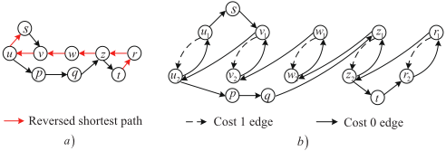
The difficulty of the algorithm is mainly in the construction of a split-residual graph ˆGwith respect to G and P ∗ , such that P ∗ ⊕Q is exactly an optimal solution to δV-2EDSP, where Q is a shortest st-path with cost at most δ in ˆG, capturing the corresponding edge-disjoint path pair in the original graph G share at most δ common vertices. Here we use P ⊕ Q to denote the set of edges P ∪ Q but with all opposite parallel edge pairs removed, where an opposite parallel edge pair is a pair of edges between an identical vertex pair but in opposite direction. The construction of the split-residual graph is similar to constructing a residual graph, except that every interior vertex on P ∗ is split and the edges are modified accordingly.
Definition 5. (Residual graph) Given a graph G with a weight function w : E → Z, P ∗ is a shortest st-path in G, the residual graph ˜G is constructed as follows. For each edge (u, v) ∈ G \ P ∗ , we add to ˜G an edge of the same weight as in G. For each edge (u, v) ∈ P ∗ , we add to ˜G a reversed edge (v, u) with a weight -w(e(u, v)).
The main steps are as below. Firstly, construct a traditional residual graph ˜G := G∪P ∗ \P ∗ , where P ∗ is the set of edges resulted from every edge on P ∗ with direction reversed and weight set negative, i.e. for every edge e = (u, v) ∈ P ∗ , add e′ = (v, u) to P ∗ with a weight w(e′ ) = -w(e). Secondly, split each interior vertex of P ∗ , say v, into two vertices v1 and v2, with an edge (v1, v2) with weight 0 and cost 1 and an edge (v2, v1) with weight 0 and cost 0, where Q going through edge (v1, v2) indicates that in G the corresponding paths resulting from P ∗ ⊕ Q will share the vertex v. Then redirect the edges that containing v: (1) replace each edge (v, u) in P ∗ by (v1, u2); (2) replace each edge (x, u) /∈ P ∗ with u ∈ P ∗ by (x, u1); (3) replace each edge (v, y) /∈ P ∗ with v ∈ P ∗ by (v2, y). Moreover, the redirected edges are with cost 0 and the same weight as the original edges. Note that the above splitting can also deal with edge (x, y) with either x ∈ P ∗ or y ∈ P ∗ . For briefness, we denote by Es the set of cost 1 edges.
The detailed construction is formally as in Algorithm 1 (An example of splitting vertices is depicted as in Figure 2).
Proposition 6. Let {P ∗ 1 , P ∗ 2 } be a spiral optimal solution to δV-2EDSP wrt G and P ∗ . Let H = P ∗ 1 ∪ P ∗ 2 ∪ P ∗ , ˆH be the split residual graph for H wrt P ∗ . Assume that Es ⊆ ˆH
is the set of edges between the pairs of split vertices for each v ∈ P ∗ . Then there must exist in ˆH an st-path Q, for which c(Q) ≤ δ and w(P ∗ ) + w(Q) ≤ w(P ∗ 1 ) + w(P ∗ 2 ) both hold.
Proof. Following Lemma 4, the set of common interior vertices of P ∗ 1 and P ∗ 2 , say V (P ∗ 1 ∩ P ∗ 2 ) \ {s, t} = {v1 , v2 , · · · , vδ }, must be all on the shortest path P ∗ . Then P ∗ 1 (vh , vh+1 ) and P ∗ 2 (vh , vh+1 ), h = 0, . . . , δ, is a pair of vertex disjoint paths between vh and vh+1 in H. We will show that there exists a path Qh ⊆ ˆH between vh 2 and vh+1 1 in ˆH with only edges of cost 0. Then there exists an st-path Q = sQ0 v1 1 v1 2 Q1 v2 1 . . . vh 1 vh 2 Qh vh+1 1 . . . vδ 1 vδ 2Qδ t, whose total cost is δ as edge (vh 1 , vh 2 ), h = 1, . . . , δ, is with cost 1 while every other edge on the path is with cost 0.
It remains only to construct Qh , ∀h. We denote the set of maximal segments in P ∗ ∩ P ∗ i (i = 1, 2) by Si = {P ∗ (xi, j, yi, j) | j = 1, . . . , hi}. W.l.o.g. assume that the first and the last maximal segments both belong to P ∗ 2 , i.e. x2, j = vh 2 and y2, h1 = vh+1 1 . Note that (x2, j, y2, j) is exactly the previous maximal segment before (x1, j, y1, j). Then we can construct Qh by using edges in ˆH only:
where x1, h+1 = t. Because the constructed Qh contains only segments of P ∗ 1 ∪ P ∗ 2 and P ∗ whose edges are of cost 0, Q is an st-path in ˆH of cost at most δ. Besides,
of edges resulting from reversing edges of P ∗ \ (S1 ∪S2). Therefore, we have w(P ∗ ) + w(Q) = w(S1) + w(S2) + w(P ∗ 1 \ S1) + w(P ∗ 2 \ S2) = w(P ∗ 1 ) + w(P ∗ 2 ). This completes the proof.
Lemma 7. Let Q be a shortest st-path with cost bounded by δ in ˆG wrt G and P ∗ , where P ∗ is a shortest st-path in G. Assume that Q′ is Q except contracting every edge between each pair of split vertices. Then P ∗ ⊕Q′ is exactly the union of two edge disjoint paths between s and t, which have a minimum total weight and share at most δ common vertices.
Proof. We will firstly show that P ∗ ⊕Q′ is exactly composed by two edge disjoint st-paths of G, which shares at most δ common vertices; secondly that w(P ∗ ⊕ Q′ ) ≤ w(OPT), where OPT is an optimal solution to δV-2EDSP.
For the first, let Q′ be Q except contracting every edge between every pair of split vertices. We need only to show the edges of P ∗ ⊕Q′ exactly compose two edge disjoint st-paths in G. First, P ∗ ∪Q′ contains an st-flow of value 2, since s and t are respectively with a degree 2 and -2 while every other vertex of P ∗ ∪Q′ \{s, t} is with degree 0. Then because P ∗ ⊕ Q′ is P ∗ ∪Q′ but removing all parallel edge pairs, P ∗ ⊕Q′ contains only edges in G. Moreover, each removed parallel edge pair is actually a cycle where each vertex is of degree 0, so in P ∗ ⊕ Q′ , s and t respectively remain degree 2 and
Algorithm 2 An exact algorithm for δV-2EDSP.
Input: A digraph G(V, E), source s and destination t, a weight function w (e), and δ ∈ Z + 0 .
Output: A solution {P1, P2} to δV-2EDSP.
- 1: Compute a shortest path P ∗ by Dijkstra's algorithm [Cormen, 2009];
- 2: Construct a split-residual graph ˆG wrt G and P ∗ by Algorithm 1;
- 3: Find a shortest path Q in ˆG with c(Q) ≤ δ by employing the algorithm for RSP as in [Joksch, 1966];
- 4: Decompose P ∗ ⊕ Q into two paths P1 and P2;
- 5: Return P1 and P2.
-2, while every other vertex remains degree 0. Therefore, P ∗ ⊕Q′ is an st-flow of value 2, and hence is a pair of edge disjoint st-path in G because each edge in P ∗ ⊕Q′ is integral.
For the common vertices, let {P1, P2} = P ∗ ⊕Q′ be the pair of disjoint st-paths. Assume that v is an interior vertex shared by P1 and P2, i.e. v ∈ P1∩P2\{s, t}. Then following the construction of the auxiliary graph as in Algorithm 1, Q has to go through the edge from v1 to v2 for the split vertex v in ˆG. Since (v1, v2) is with cost 1 and every other edge is with cost 0, Q can at most go through δ such edges between split vertex pair as it has a cost no larger than δ. Therefore, P1 and P2 share at most δ common vertices.
For the second, from Theorem 3, there must exist a spiral optimal solution to δV-2EDSP, say {P ∗ 1 , P ∗ 2 }. Let H = P ∗ 1 ∪ P ∗ 2 ∪ P ∗ and ˆH be the accordingly residual graph wrt P ∗ . Then from Proposition 6, we can obtain an st-path Q′′ in ˆH with c(Q′′ ) ≤ δ and w(P ∗ ) + w(Q′′ ) ≤ w(P ∗ 1 ) + w(P ∗ 2 ). Since ˆH ⊆ ˆG, Q′′ is also an st-path in ˆGwith both c(Q′′ ) ≤ δ and w(P ∗ )+w(Q′′ ) ≤ w(P ∗ 1 )+w(P ∗ 2 ) = w(OPT ). Then because Q is the shortest path in ˆG, we have w(Q) ≤ w(Q′′ ), and hence w(P ∗ )+w(Q) ≤ w(OPT ) holds. This completes the proof.
Following the above construction, we can obtain a splitresidual graph ˆG = ( ˆ V , ˆE), where the δV-2EDSP problem is transformed to the problem of finding a minimum weight st-path with cost bounded by δ, namely the Binary Restricted Shortest Path (BRSP) problem, which is clearly a special case of the restricted shortest path (RSP) problem. Following the algorithm for RSP [Joksch, 1966], the BRSP problem can be solved in time O(δ|E|) by employing the dynamic programming method. Thus, Q can be computed within time O(δ|E|). Then following Lemma 7, P ∗ ⊕Q′ exactly composes an optimal solution to δV-2EDSP, where Q′ is Q contracting each pair of split vertices back to one vertex in G, say contracting v1 and v2 to v. The formal layout of the whole algorithm is as in Algorithm 2.
Lemma 8. Algorithm 2 runs in time O(δm+ n log n).
Proof. Let m = |E(G)| and n = |V (G)|. Then, the algorithm takes O(m + n log n) time to run Dijkstra's algorithm against the original graph G in Step 1 [Cormen, 2009], and O(m+n) time to construct a split- residual graph ˆG in Step 2. In Step 3, the algorithm for BRSP runs in O(mδ), where δ is the bound of the number of common vertices. Other steps obviously takes trivial time comparing to the above ones. Therefore, the total runtime of Algorithm 2 is O(δm+n log n).
Combining Lemma 7 and 8, we immediately have the following theorem:
Theorem 9. Algorithm 2 runs in time O(δm+ n log n) and outputs an optimal solution to δV-2EDSP.
3 Experimental Results
In this section, we shall first evaluate the practical performance of Algorithm 2 (the exact algorithm, denoted as EA) by comparing its runtime and solution quality with another two algorithm baselines: the best previous algorithm (PA) presented in [Yallouz et al., 2016], and an exact algorithm via solving a flow integer linear program (ILP) formulation 1 we designed for δV-2EDSP. Then we show EA is scalable by running it against real-world network data including communication networks and P2P networks from Stanford Large Network Dataset Collection 2 within Stanford Network Analysis Project (SNAP). These algorithms are implemented in Python 2.7 (The code is available upon request), on a PC with Intel Core i5 processor, and 8GB memory. Our implementation adopts the NetworkX library 3 to construct and process graphs, the GLPK library 4 to solve the ILP.
3.1 Simulation Results
In this subsection, we evaluate the runtime of the algorithms by simulation experiments, in which we generate a random graph from NetworkX with n vertices, and m edges each with a weight uniformly distributed in [1, 100]. The number of allowed common vertices is the parameter δ.
Simulation results comparing runtimes of EA, PA and ILP in seconds are depicted in Table 1. For each row of the table, we first randomly generated 1000 different graphs of the given size (n,m), then respectively ran the three algorithms against each graph given a randomly chosen source and destination node pair, and at last computed the average time over the 1000 runs. Notice that during runs, the encountered infeasible graph instances do not contribute to our average time calculations. In the experiments, when the problem size is not larger than n = 100 and m = 1000, the runtime of EA is close to that of ILP 5 , but significantly faster than PA, say, about a thousand times faster. This matches the theoretical runtime difference between EA and PA, i.e. O(δm+n log n) vs O(mn2 + n3 log n). When the problem size grows larger, PA quickly becomes not scalable as it takes too long to produce a solution. So for larger graphs we only compared the runtimes of EA and ILP. The simulation results show that EA
1 The formulation is available upon request but was omitted here due to space limit.
2 https://snap.stanford.edu/data/
3 https://networkx.github.io/
4 https://www.gnu.org/software/glpk/
5 Most likely because the random graph structure with a small n becomes easier for the solution search of ILP solver that usually runs in worst case exponential time in n.
| Size (n, m, δ) | EA (s) | PA (s) | ILP (s) | Size (n, m, δ) | EA (s) | ILP (s) |
|---|---|---|---|---|---|---|
| (50, 250, 5) | 0.023 | 7.843 | 0.029 | (500, 25000, 10) | 0.720 | 1.067 |
| (55, 302, 6) | 0.026 | 10.404 | 0.031 | (550, 30250, 10) | 1.0923 | 1.476 |
| (60, 5360, 6) | 0.03 | 14.515 | 0.032 | (600, 36000, 10) | 1.240 | 1.871 |
| (65, 422, 6) | 0.033 | 20.381 | 0.034 | (650, 42250, 10) | 1.344 | 2.552 |
| (70, 490, 6) | 0.035 | 26.468 | 0.035 | (700, 49000, 10) | 1.536 | 3.392 |
| (75, 562, 8) | 0.041 | 34.255 | 0.047 | (750, 56250, 10) | 1.603 | 3.554 |
| (80, 640, 8) | 0.044 | 43.820 | 0.051 | (800, 64000, 12) | 1.906 | 4.529 |
| (85, 722, 8) | 0.053 | 54.767 | 0.061 | (850, 72250, 12) | 2.200 | 5.688 |
| (90, 810, 10) | 0.075 | 68.818 | 0.074 | (900, 81000, 12) | 2.468 | 7.459 |
| (95, 902, 10) | 0.080 | 85.434 | 0.084 | (950, 90250, 12) | 2.805 | 8.492 |
| (100, 1000, 10) | 0.090 | 104.518 | 0.095 | (1000, 100000, 12) | 3.041 | 10.039 |
| Networks | #Nodes | #Edges | EA (s) | Networks | #Nodes | #Edges | EA (s) |
|---|---|---|---|---|---|---|---|
| Email-Enron | 36,692 | 183,831 | 20.76 | p2p-Gnut.09 | 8,114 | 26,013 | 2.40 |
| Email-EuAll | 265,214 | 420,045 | 35.04 | p2p-Gnut.24 | 26,518 | 65,369 | 6.02 |
| p2p-Gnut.05 | 8,846 | 31,839 | 2.55 | p2p-Gnut.25 | 22,687 | 54,705 | 5.13 |
| p2p-Gnut.06 | 8,717 | 31,525 | 2.94 | p2p-Gnut.30 | 36,682 | 88,328 | 8.44 |
| p2p-Gnut.08 | 6,301 | 20,777 | 1.92 | p2p-Gnut.31 | 62,586 | 147,892 | 13.40 |
still runs much faster than ILP and more importantly the gap between these two grows with graph size.
It is also worth mentioning that, when testing against the same graph, the min-sum weights of the solutions, produced by all three algorithms, coincide in all experiments on the generated thousands of graphs. It was known that ILP and PA always output optimal solutions, so this observation can be regarded as an experimental evidence that our EA also produces optimal solutions, complementing our optimality proof.
3.2 Real-world Evaluation
Besides simulation results, we also ran EA against some realworld network datasets from the SNAP collections. In the experiment, we ran EA for 200 times and each time we instead randomly pick two vertices in the network as source and destination. We again report the average runtime for EA. We also reasonably set δ = 10, because in real networks, many protocols (TCP/IP etc.) only allow a data package pass through at most 16 routers from source to destination [Kurose and Ross, 2009]. Therefore a shortest path for transmitting data will have at most 16 interior vertices in most cases.
The experimental results depicted in Table 2 show that, roughly the runtime of EA is linearly dependent on the number of edges of the network. Moreover, EA takes up to 35 seconds to process a network with 265k nodes and 420k edges whereas PA and ILP in our experiments can not even complete in many hours. Also noting that, although currently EA takes tens of seconds to process median size networks, it can be significantly accelerated with a more sophisticated C/C++ implementation and a higher end computing platform. These together will allow EA to efficiently process much larger graphs with hundreds of millions of nodes and edges. This is also supported from the time complexity of EA that is almost linear in the network size.
4 Conclusion
In this paper, we carried on studying the problem of finding minimum-weight k edge-disjoint partially vertex-disjoint paths, namely δV-kEDSP. We proposed an optimal algorithm for δV-2EDSP that efficiently runs in O(δm+ n logn) time and in experiments demonstrates a significant runtime gain. This greatly improves the previous best runtime bound of O(mn2 + n3 logn) [Yallouz et al., 2016], where m, n and δ are respectively the number of edges, vertices and allowed shared vertices. Note that the time complexity of our algorithm flexibly depends on δ, which is at most n (though a fixed δ is more practical), so the worst-case complexity is O(mn+n log n) - still a much better bound. We are currently investigating solving δV-kEDSP by extending our technique for δV-2EDSP. Also we are considering the counterpart problem δE-kEDSP, in which the number of edges shared by at least two paths is bounded by δ instead.
Acknowledgements
The research is supported by Natural Science Foundation of China (Nos. 61772005, 61300025) and Natural Science Foundation of Fujian Province (No. 2017J01753).
@inproceedings{ijcai2018p202,
  title     = {A Fast Algorithm for Optimally Finding Partially Disjoint Shortest Paths},
  author    = {Guo, Longkun and Deng, Yunyun and Liao, Kewen and He, Qiang and Sellis, Timos and Hu, Zheshan},
  booktitle = {Proceedings of the Twenty-Seventh International Joint Conference on
               Artificial Intelligence, {IJCAI-18}},
  publisher = {International Joint Conferences on Artificial Intelligence Organization},
  editor    = {Jérôme Lang},
  pages     = {1456--1462},
  year      = {2018},
  month     = {7},
  note      = {Main track},
  doi       = {10.24963/ijcai.2018/202},
  url       = {https://doi.org/10.24963/ijcai.2018/202},
}
TY - CPAPER TI - A Fast Algorithm for Optimally Finding Partially Disjoint Shortest Paths AU - Guo, Longkun AU - Deng, Yunyun AU - Liao, Kewen AU - He, Qiang AU - Sellis, Timos AU - Hu, Zheshan T2 - Proceedings of the Twenty-Seventh International Joint Conference on Artificial Intelligence, IJCAI-18 PB - International Joint Conferences on Artificial Intelligence Organization PY - 2018 SP - 1456 EP - 1462 DO - 10.24963/ijcai.2018/202 UR - https://doi.org/10.24963/ijcai.2018/202 ER -Copied
Machine-readable versions of this paper, for tools and AI agents:





