
Learn the Highest Label and Rest Label Description Degrees
Proceedings of the Thirtieth International Joint Conference on Artificial Intelligence. Main Track. Pages 3097-3103.
https://doi.org/10.24963/ijcai.2021/426
Keywords
- Machine Learning: Multi-instance; Multi-label; Multi-view learning
- Machine Learning: Structured Prediction
Abstract
Although Label Distribution Learning (LDL) has found wide applications in varieties of classification problems, it may face the challenge of objective mismatch -- LDL neglects the optimal label for the sake of learning the whole label distribution, which leads to performance deterioration. To improve classification performance and solve the objective mismatch, we propose a new LDL algorithm called LDL-HR. LDL-HR provides a new perspective of label distribution, \textit{i.e.}, a combination of the \textbf{highest label} and the \textbf{rest label description degrees}.
It works as follows. First, we learn the highest label by fitting the degenerated label distribution and large margin. Second, we learn the rest label description degrees to exploit generalization. Theoretical analysis shows the generalization of LDL-HR. Besides, the experimental results on 18 real-world datasets validate the statistical superiority of our method.
- [Bartlett and Mendelson, 2002] Peter L. Bartlett and Shahar Mendelson. Rademacher and gaussian complexities: Risk bounds and structural results. Journal of Machine Learn- ing Research, 3(9):463-482, 2002.
- [Berger et al., 1996] Adam L. Berger, Stephen A. Della Pietra, and Vincent J. Della Pietra. A maxi- mum entropy approach to natural language processing. Computational Linguistics, 22(1):39-71, March 1996.
- [Chang and Lin, 2011] Chih-Chung Chang and Chih-Jen Lin. Libsvm: A library for support vector machines. ACM Transactions on Intelligent Systems and Technology, 2(3):1-27, May 2011.
- [Cortes and Vapnik, 1995] Corinna Cortes and Vladimir Vapnik. Support-vector networks. 20(3):273-297, September 1995.
- [Demšar, 2006] Janez Demšar. Statistical comparisons of classifiers over multiple data sets. Journal of Machine Learning Research, 7(1):1-30, 2006.
- [Devroye et al., 1996] Luc Devroye, László Györfi, and Gábor Lugosi. A Probabilistic Theory of Pattern Recog- nition, volume 31 of Stochastic Modelling and Applied Probability. Springer, 1996.
- [Gao et al., 2017] Binbin Gao, Chao Xing, Chenwei Xie, Jianxin Wu, and Xin Geng. Deep label distribution learn- ing with label ambiguity. IEEE Transactions on Image Processing, 26(6):2825-2838, March 2017.
- [Gao et al., 2018] Binbin Gao, Hongyu Zhou, Jianxin Wu, and Xin Geng. Age estimation using expectation of la- bel distribution learning. In Proceedings of the 27th Inter- national Joint Conference on Artificial Intelligence, pages 712-718, August 2018. IJCAI
- [Geng and Hou, 2015] Xin Geng and Peng Hou. Pre-release prediction of crowd opinion on movies by label distribu- tion learning. In Proceedings of the 24th International Conference on Artificial Intelligence, page 3511-3517, July 2015. IJCAI
- [Geng and Xia, 2014] Xin Geng and Yu Xia. Head pose es- timation based on multivariate label distribution. In Pro- ceedings of IEEE Conference on Computer Vision and Pat- tern Recognition, pages 1837-1842, June 2014.
- [Geng, 2016] Xin Geng. Label distribution learning. IEEE Transactions on Knowledge and Data Engineering, 28(7):1734-1748, March 2016.
- [Jia et al., 2019] Xiuyi Jia, Xiang Zheng, Weiwei Li, Changqing Zhang, and Zechao Li. Facial emotion distri- bution learning by exploiting low-rank label correlations locally. In Proceedings of the IEEE/CVF Conference on Computer Vision and Pattern Recognition, pages 9833- 9842, June 2019.
- [Jia et al., 2021] Xiuyi Jia, Zechao Li, Xiang Zheng, Weiwei Li, and Shengjun Huang. Label distribution learning with label correlations on local samples. IEEE Transactions on Knowledge and Data Engineering, 33(4):1619-1631, April 2021.
- [Li and Deng, 2019] Shan Li and Weihong Deng. Blended emotion in-the-wild: Multi-label facial expression recog- nition using crowdsourced annotations and deep locality feature learning. International Journal of Computer Vi- sion, 127(6-7):884-906, November 2019.
- [Liang et al., 2018] Lingyu Liang, Luojun Lin, Lianwen Jin, Duorui Xie, and Mengru Li. SCUT-FBP5500: A diverse benchmark dataset for multi-paradigm facial beauty pre- diction. In Proceedings of the 24th International Con- ference on Pattern Recognition, pages 1598-1603, August 2018.
- [Nguyen et al., 2012] Tam V. Nguyen, Si Liu, Bingbing Ni, Jun Tan, Yong Rui, and Shuicheng Yan. Sense beauty via face, dressing, and/or voice. In Proceedings of the 20th ACM International Conference on Multimedia, page 239-248, October 2012.
- [Nocedal and Wright, 2006] Jorge Nocedal and Stephen J. Wright. Numerical optimization. Springer series in op- erations research and financial engineering. Springer, New York, 2rd. edition, 2006.
- [Ren and Geng, 2017] Yi Ren and Xin Geng. Sense beauty by label distribution learning. In Proceedings of the 26th International Joint Conference on Artificial Intelligence, pages 2648-2654, August 2017. IJCAI
- [Rupprecht et al., 2017] Christian Rupprecht, Iro Laina, Robert DiPietro, Maximilian Baust, Federico Tombari, Nassir Navab, and Gregory D. Hager. Learning in an un- certain world: Representing ambiguity through multiple hypotheses. In Proceddings of IEEE International Con- ference on Computer Vision, pages 3611-3620, October 2017.
- [Shen et al., 2017] Wei Shen, Zhao Kai, Yilu Guo, and Alan L. Yuille. Label distribution learning forests. In Advances in Neural Information Processing Systems 30, pages 834-843. December 2017.
- [Wang and Geng, 2019] Jing Wang and Xin Geng. Classifi- cation with label distribution learning. In Proceedings of the 28th International Joint Conference on Artificial Intel- ligence, pages 3712-3718, August 2019. IJCAI
- [Xie et al., 2015] Duorui Xie, Lingyu Liang, Lianwen Jin, Jie Xu, and Mengru Li. SCUT-FBP: A benchmark dataset for facial beauty perception. In Proceedings of IEEE In- ternational Conference on Systems, Man, and Cybernetics, pages 1821-1826, October 2015.
- [Yang et al., 2017] Jufeng Yang, Dongyu She, and Ming Sun. Joint image emotion classification and distribution learning via deep convolutional neural network. In Pro- ceedings of the 26th International Joint Conference on Ar- tificial Intelligence, pages 3266-3272, August 2017. IJCAI
- [Zhang and Zhou, 2014] Minling Zhang and Zhihua Zhou. A review on multi-label learning algorithms. Transactions on Knowledge and Data Engineering, 26(8):1819-1837, August 2014.
References were extracted automatically from the PDF and may contain errors.
Full text extracted automatically from the PDF; figures, tables and equations may differ. The PDF is the version of record.
1 Introduction
In traditional supervised learning paradigms, such as SingleLabel Learning (SLL) and Multi-Label Learning (MLL), the relation between instances and labels is deterministic: 0 for relevant and 1 for irrelevant [Zhang and Zhou, 2014]. Nevertheless, in many real-world scenarios, label ambiguity is widespread [Gao et al., 2017], i.e., the relation between instances and labels contains some uncertainty [Rupprecht et al., 2017], which may limit the applications of SLL and MLL. To address that, Geng [2016] proposes a new learning paradigm called Label Distribution Learning (LDL). Instead of 0/1 labels, LDL annotates each instance with a label distribution. A label distribution is a vector of real-values whose elements are called the label description degrees that specify the relative importance of labels to instances. LDL can handle label ambiguity and attracts lots of attention.
As an effective solution to label ambiguity, LDL has seen many classification applications such as age estimation [Shen et al., 2017], head-pose estimation [Geng and Xia, 2014], sentiment analysis [Yang et al., 2017], emotion recognition
∗Corresponding author.
[Li and Deng, 2019], beauty perception [Liang et al., 2018], etc. Generally, applications of LDL involve two phases. First, in the training phase, an LDL function is learned from the training set with label distributions. Second, in the test phase, the learned LDL function is regarded as a classifier - for an unknown instance, the label that has the highest predicted label description degree by the learned LDL function is regarded as the predicted label. Take head-pose estimation [Geng and Xia, 2014] as an example. First, an LDL function is learned from the pose images described by label distributions. Then, for an unknown image, the pose label that has the highest predicted label description degree is considered as the predicted pose.
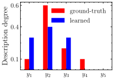
Although LDL has found wide classification applications, it faces the challenge of objective mismatch [Wang and Geng, 2019; Gao et al., 2018]. That is, the objective of LDL mismatches that of classification. The objective of LDL is to learn the whole label distribution, while the goal of classification is to learn the optimal label - LDL may neglect the optimal label for the sake of learning the whole label distribution. Fig. 1 explains the objective mismatch by examples. Even though the learned LDL function of Fig. 1a has a smaller L1-norm loss, the predicted label (y2) is different from the optimal one (y1). The learned LDL function of Fig. 1b has a larger L1-norm loss but the predicted label (y2) equals the optimal one (y2). Gao et. al [2018] first pointed out the objective mismatch in age estimation. Wang and Geng [2019] designed a specialized LDL algorithm to alleviate the objective mismatch. Besides these two, existing works on LDL seldom notice the objective mismatch.
To solve the objective mismatch, we propose in this paper a new LDL method called LDL-HR. We view label distribution equivalently as a combination of the highest label (i.e., the label with the highest description degree) and the rest label description degrees (i.e., all description degrees except that of the highest label). We prove that both the highest label and the rest label description degrees are necessary for the generalization of LDL (Theorems 1 and 2). Inspired by that, LDL-HR jointly learns the highest label and the rest label description degrees. We conduct extensive experiments on 18 real-world datasets. The experimental results show the better classification performance of LDL-HR. Further analysis validates the usefulness of learning the highest label and the rest label description degrees.
Description degree
0.4
0.3
0.2
0.1
ground-truth
learned
y1
y2
y3
y4
y5
(a) L1-norm loss: 0.2; 0/1 loss: 1
(b) L1-norm loss: 0.6; 0/1 loss: 0
Figure 1: Illustration of the objective mismatch. For (a), the learned LDL function has a smaller L1-norm loss while the predicted label (y2) is different from the optimal one (y1). However, for (b), the predicted LDL function has a larger L1-norm loss but the predicted label (y2) equals the optimal one (y2).
Our contributions are as follows. First, we present a novel perspective of label distribution - a combination of the highest label and the rest label description degrees. Theoretical findings show that both the highest label and the rest label description degrees are necessary for the generalization of LDL algorithms. Second, we propose a new LDL method LDLHR. Inspired by the theoretical findings, LDL-HR jointly learns the highest label and the rest label description degrees. Experimental results validate the effectiveness of LDL-HR.
2 Preliminaries
2.1 Notations
Denote by X ⊂ Rq the input space and Y = {y1, · · · , ym} the label space. Each x ∈ X is annotated with a label distribution D = [dy1 x , · · · , dym x ]⊤, where dyj x is called the label description degree and satisfies dyj x ≥ 0 and ∑mj=1 dyj x = 1 [Geng, 2016]. Given a training set with n examples S = {(x1,D1), (x2,D2), · · · , (xn,Dn)}, the goal of LDL is to learn a multi-output function p : X → Rm which minimizes the difference between the outputs of p and the ground-truth label distributions [Geng, 2016].
Let ‖ · ‖2 and ‖ · ‖F respectively denote the L2-norm and Frobenius norm, and [m] be the set {1, · · · ,m}. Let sign(·) be the sign function and I(·) be the indicator function. Let D be the (unknown) underlying distribution over X . Define
i.e., the highest label that has the optimal label description degree. Let y ∈ Y be the random label variable. Suppose that the label distribution function is the conditional probability distribution function, i.e., dyj x = P(y = yj|x). Let L∗1 be the Bayes error [Devroye et al., 1996].
2.2 LDL and Classification
Classification with LDL can be formulated as follows. First, an LDL function h is learned from S by optimizing
where W is the parameter, and ℓ is a loss function. Second, a classifier is definedf(x) = argmax
where h ¯ yx is the predicted label description degree of ¯ y to x. That is, the label having the highest predicted label description degree by h is regarded as the predicted label. The goal of LDL-HR is to minimize the error P(f(x) ̸= y).
3 The LDL-HRMethod
This section explains the proposed method. First, we address the objective mismatch by learning the highest label. Second, we learn the rest label description degrees to exploit generalization. Third, we elaborate on the optimization method.
3.1 Learn the Highest Label
As discussed in Section 1 that LDL faces the challenge of objective mismatch when adopted to classification problems. To alleviate that, we learn the highest label by learning the degenerated label distribution and large margin.
To start, we define the degenerated label distribution. Specifically, for each x, define ¯D = [ ¯ dy1 x , ¯ dy2 x , · · · , ¯ dym x ]⊤, where ¯ dyj x is defined by
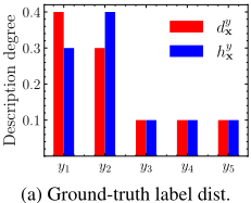
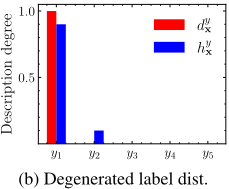
That is, we assign a degree of 1 to the highest label and 0s to other labels. When learning the degenerated label distribution, an LDL model would mainly focus on the highest label because the label description degree of the highest label dominates those of other labels. Thereby, the degenerated label distribution is helpful to alleviate the objective mismatch. Fig. 2 shows an example of learning the ground-truth and the degenerated label distributions, where the red bars are the ground-truth and the degenerated distributions, and the blue bars are the learned distributions. From Fig. 2, we can see that i) the learned LDL functions of both (a) and (b) achieve L1-norm losses of 0.2, and ii) the predicted label of (b) (y1) equals the optimal label (y1) while the predicted label of (a) (y2) doesn't, which shows the advantage of learning the degenerated label distribution. Besides, learning the degenerated label distribution also has theory guarantee, which is shown by the next theorem.
Theorem 1. Let ¯D be the degenerated label distribution as defined in Eq. (4). Let h be a learned LDL function, and f be the classifier as defined in Eq. (3). Then, the expected 0/1 loss of f satisfies the following bound
Theorem 1 says that the expected 0/1 loss of a classifier would approach the Bayes error if the outputs of the learned LDL function is close to the degenerated label distribution in L1-norm distance sense. That is, to learn a classifier with small 0/1 loss, it suffices to minimize the L1-norm distance between the LDL function and the degenerated distribution.
By Theorem 1, we use L1-norm loss to learn the degenerated label distribution. Similar to [Geng, 2016], we adopt the maximum entropy model [Berger et al., 1996] defined by
Then, LDL can be cast as the following optimization problem
whereW = [w1, · · · ,wm] is the model parameter, and λ1 is the regularization parameter.
Next, we borrow large margin theory [Cortes and Vapnik, 1995] to further improve classification performance. Our basic idea is to encourage the predicted label description degree of the highest label to be larger than those of other labels by a margin ρ > 0. Then, the predicted label would be consistent with the highest one, which alleviates the objective mismatch. Recall the highest label yxi = argmax¯ y d ¯ yxi . Adding large margin to Eq. (6), we have the next optimization problem
where ξi,j is a slack variable, and λ2 is a trade-off parameter. The constraints encourage the predicted label description degree of yxi to be larger than those of other labels by ρ.
3.2 Learn the Rest Label Description Degrees
Observe that model (7) only learns the highest label and neglects the rest label description degrees (i.e., the label description degrees of all labels except the highest one), which loses lots of supervision information. As shown in Fig. 2 that, the ground-truth label distribution has much more supervision information than the degenerated one, particularly for the labels except the highest label. Indeed, the rest label description degrees are necessary for the generalization of LDL. Concretely, let f ′ be the sub-optimal classifier defined by
which outputs the highest label in the rest label description degrees (the label with the second highest label description degree). Define the expected 0/1 loss of f ′ by L∗2 = P(f ′ (x) ̸= y). The next theorem shows the generalization of LDL w.r.t. learning the rest label description degrees.
Theorem 2. Let h be a learned LDL function, and f be the classifier as defined in Eq. (3). Then, the expected 0/1 loss of f satisfies the following bound
Theorem 2 says that the expected 0/1 loss of the classifier can be bounded by the sum of two items. The first one is the expected 0/1 loss of the sub-optimal classifier, and the second one is the expected L1-norm distance between the outputs of the learned LDL function and the rest label description degrees. In another word, even if the expected 0/1 loss of the classifier doesn't reach the Bayes error, it can still be bounded by that of the sub-optimal classifier as long as the outputs of the learned LDL function is close to the rest label description degrees in L1-norm distance sense. By Theorem 2, we learn the rest label description degrees with L1-norm loss to exploit generalization, and re-cast Eq. (7) as the following
where λ3 is a trade-off parameter, and the last item learns the rest label description degrees. We defer the proofs for the theorems to the Supplementary Material 1 .
3.3 Optimization
It's challenging to solve Eq. (10) directly due to the large number of constraints (2n(m - 1) constraints). Here, we solve it by iterative methods. Define ℓρ(x) = max{0, 1 - x/ρ}. Then, Eq. (10) can be equivalently re-written as
Define ωi,j = sign(hyj x - ¯ dyj x ), ¯ωi,j = sign(hyj x - dyj x ), and ˆωi,j = I(hyxi xi - hyj xi ≤ ρ). The gradient of the preceding objective function can be obtained through
where the gradient of maximum entropy can be calculated as
Since the problem is a convex optimization problem, a quasiNewton algorithm L-BFGS [Nocedal and Wright, 2006] is applied to efficiently solve it.
1 Available at: https://github.com/wangjing4research/LDL HR
4 Generalization
This section analyzes the generalization of LDL-HR. For an LDL function h, let f be the classifier defined in Eq. (3). Next, define ˆR(h) = 1n ∑i,j |hyj xi - ¯ dyj xi |, ¯R(h) = 1n ∑i,j:yj ̸=yxi |hyj xi - dyj xi |, and the error R(h) = P(f(x) ̸= y). Let SF be the softmax function. For simplicity, let supx∈X ‖x‖2 ≤ Λ1 for a constant Λ1 > 0.
Theorem 3. Define F = {x ↦→W ⊤x | ‖wj‖2 ≤ Λ2, ∀j ∈ [m]} and H = {x ↦→ SF(g(x)) | g ∈ F}2 . Then, for any δ > 0, with probability at least 1 - δ, the following bound holds for all h ∈ H
Theorem 3 bounds the error by the sum of four items. The first one is the empirical L1-norm loss, the second is an upper bound on the Rademacher complexity [Bartlett and Mendelson, 2002] for H, the third one is an empirical estimation of the Bayes error, and the last one can be ignored. Next, let y′x = f ′ (x), where f ′ is defined in Eq. (8).
Theorem 4. Let H be the hypothesis space defined in Theorem 3. For any δ > 0, with probability at least 1 - δ, the following bound holds for all h ∈ H
Theorem 4 bounds the error by the sum of four items, where the first one is the empirical L1-norm loss w.r.t. the rest label description degrees, the second one bounds the complexity of H, the third one is an empirical estimation of the generalization error of f ′ . By Theorems 3 and 4, both the highest label and the rest label description degrees are helpful for the generalization of our model.
5 Experiments
5.1 Methodology
Experimental Datasets. Table 1 summarizes the statistics of the experimental datasets. The first 15 datasets (from Alpha to SBU 3DFE) are collected by Geng [2016]. The last three datasets M2B [Nguyen et al., 2012], SCUT-FBP [Xie et al., 2015], and fbo5500 [Liang et al., 2018] are about facial beauty perception. For M2B, the label distributions are transformed from k-wise comparisons [Ren and Geng, 2017]. For fbp5500, we use the trained ResNet to extract 512dimensional features. In the sequel, each dataset is denoted by its first three letters (Spoem and Spo5 are denoted by Spoe and Spo5 to distinguish them from Spo).
EvaluationMetrics. Our motivation is to improve the classification performance and solve the objective mismatch of LDL. Hence, the commonly used LDL metrics are not used. To evaluate the classification performance of algorithms, we regard the highest label (i.e., yx) as the ground-truth label and use 0/1 loss, i.e., ℓ0/1(f(x), yx) = I(f(x) ̸= yx). To further analyze the generalization ability of algorithms, we use the error probability proposed in [Wang and Geng, 2019]. Let ¯ y = f(x), then the error probability is defined by
2 The maximum entropy model is equivalent to a functional combination of the softmax function and a linear function.
| ID. | Dataset | #Examples | #Features | #Labels |
|---|---|---|---|---|
| 1 | Alpha | 2,465 | 24 | 18 |
| 2 | Cdc | 2,465 | 24 | 15 |
| 3 | Cold | 2,465 | 24 | 4 |
| 4 | Diau | 2,465 | 24 | 7 |
| 5 | Dtt | 2,465 | 24 | 4 |
| 6 | Elu | 2,465 | 24 | 14 |
| 7 | Heat | 2,465 | 24 | 6 |
| 8 | Spo | 2,465 | 24 | 6 |
| 9 | Spo5 | 2,465 | 24 | 3 |
| 10 | Spoem | 2,465 | 24 | 2 |
| 11 | Scene | 2,000 | 294 | 9 |
| 12 | Gene | 17,892 | 36 | 68 |
| 13 | Movie | 7,755 | 1,869 | 5 |
| 14 | SJAFFE | 213 | 243 | 6 |
| 15 | SBU 3DFE | 2,500 | 243 | 6 |
| 16 | M2B | 1,240 | 250 | 5 |
| 17 | SCUT-FBP | 1,500 | 300 | 5 |
| 18 | fbp5500 | 5,500 | 512 | 5 |
Baselines. We compare LDL-HR against seven methods, details of which are summarized as follows.
- Logistic Regression (LR): the maximum entropy model can be viewed as a multi-nomial LR. Accordingly, we compare LDL-HR against LR.
- Support Vector Machine (SVM) [Chang and Lin, 2011]: LDL-HR uses large margin, which can be viewed as an SVM. Here, one-vs-rest SVM is compared against.
- SA-BFGS [Geng, 2016]: it uses the maximum entropy model to learn label distribution, where KL divergence is employed as the learning metric.
- LDL-SVR [Geng and Hou, 2015]: it adopts the multioutput Support Vector Regression (SVR) model to learn label distribution.
- EDL-LRL [Jia et al., 2019]: it exploits the local lowrank structure of label distribution to consider local label correlation when learning label distribution.
- LDL-SCL [Jia et al., 2021]: it encodes label correlations as additional features, and jointly learns label distribution and label correlation.
- LDL4C [Wang and Geng, 2019]: it's a specialized LDL method for classification with label distribution, where instances are weighted and large margin is used.
Parameter Settings. The parameters of the baselines are set as follows. For SVM and LDL-SVR, the linear kernel is used and C = 1. For LDL-SVR, ϵ = 0.1. For SABFGS, EDL-LRL, and LDL-SCL, the default parameters are used. For LDL4C, C1 and C2 are selected from the candidate set {10-3 , · · · , 103 } and ρ is selected from the pool {0.001, 0.01, 0.1}. For LDL-HR, λ1 = 0.001, λ2 and λ3 are tuned from the candidate set {10-3 , · · · , 1}, and ρ = 0.01. We first tune the parameters of each method by 10-fold crossvalidation, and then run each method with the best parameters for 10 times random data partitions (90% for training and 10% for testing). The mean performance and the standard deviation are reported.
5.2 Results and Discussion
Tables 2 and 3 tabulate the experimental results of each comparing method in terms of 0/1 loss and error probability, respectively. The best results are highlighted in boldface. Further, we conduct the pairwise t-test at a confidence of 0.05 and use ·/◦ to indicate whether LDL-HR is statistically superior/inferior to the comparing methods.
According to Tables 2 and 3, LDL-HR ranks first in 72.2% and 77.8% cases in terms of 0/1 loss and error probability respectively, and achieves significantly superior performance against other methods in 64.3% and 52.4% cases in terms of 0/1 loss and error probability, respectively. LDL-HR is comparable to LR and SVM in terms of 0/1 loss, and outperforms them by a large margin in terms of error probability, which implies the better generalization of LDL-HR. The reason is that LDL-HR learns, besides the highest label, the rest label description degrees, which is consistent with our theoretical finding (Theorem 2). Compared with SA-BFGS, LDLSVR, EDL-LRL, and LDL-SCL, LDL-HR achieves statistically better performance in terms of 0/1 loss and comparable performance in terms of error probability. On one hand, LDL-HR solves the objective mismatch and has better classification performance by learning the highest label. On the other hand, LDL-HR achieves comparable generalization to the LDL algorithms by learning the rest label description degrees. Moreover, LDL-HR achieves comparable performance to LDL4C with the win/tie/lose counts of 7/11/0 and 2/16/0 in terms of 0/1 loss and error probability, respectively. It's noteworthy that LDL-HR has much better mean performance (top-1 times of 13 and 14) than LDL4C (top-1 times of 4 and 8) for both 0/1 loss and error probability.
5.3 Parameter Sensitivity Analysis
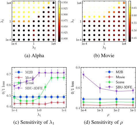
LDL-HR has four parameters, including the regularization parameter λ1, the trade-off parameters λ2 and λ3, and the margin ρ. To show the robustness of λ1, λ2, and λ3, we tune them from {10-4 , · · · , 104 }. Fig. 3a and 3b show the results of the grid-search for λ2 and λ3 on Alpha, Movie in terms of 0/1 loss. Accordingly, λ2 = 0.1 and λ3 = 0.1 bring satisfying performance. Fig. 3c presents the sensitivity of λ1 on M2B, Movie, Scene, and SBU 3DFE. By Fig. 3c, LDL-HR with λ1 = 0.001 has better performance. To show the sensitivity of ρ, we tune it from the set {10-4 , · · · , 10-1 }. Fig. 3d shows the sensitivity of ρ . We can see from Fig. 3d that LDL-HR is robust w.r.t. ρ, which can be set to 0.01.
5.4 Ablation Study
We conduct ablation studies to analyze the usefulness of learning the highest label and the rest label description degrees. We first derive a degenerated version LDL-H that only considers the highest label by setting λ2 = 0 and λ3 = 0.
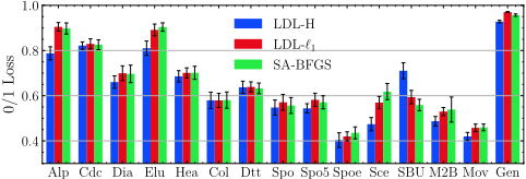
LDL-H only learns the degenerated label distribution. To see the effectiveness of that, we replace the degenerated label distribution with the ground-truth one, and denote the method by LDL-ℓ1 (learns the ground-truth label distribution with L1-norm loss). We compare LDL-H with LDL-ℓ1. Besides, we also compare LDL-H with SA-BFGS that only differs from LDL-H in learning the ground-truth label distribution with KL divergence. Fig. 4 presents the detailed results of LDL-H, LDL-ℓ1, and SA-BFGS in terms of 0/1 loss on some datasets. To show the usefulness of learning the rest label description degrees, we compare LDL-HR (with λ2 = 0) against LDL-H since they are only different in that LDL-H ignores the rest label description degrees. We further conduct the Wilcoxon signed-rank tests [Demˇsar, 2006] for LDL-H against LDL-ℓ1 and SA-BFGS, and LDL-HR against LDLH, which are reported in Table 4 (win/tie/lose at 0.05 significance level). According to Table 4, learning the highest label brings statistically better classification performance, and learning the rest label description degrees leads to statistically superior generalization.
| LR | SVM | SA-BFGS | LDL-SVR | EDL-LRL | LDL-SCL | LDL4C | LDL-HR | |
|---|---|---|---|---|---|---|---|---|
| Alp | 79.07±2.90• | 78.74±2.91 | 89.74±2.47• | 90.83±2.02• | 89.70±2.37• | 91.24±1.73• | 78.70±2.34 | 78.30±3.06 |
| Cdc | 82.47±2.36 | 82.47±2.25 | 82.56±2.20 | 82.43±1.99 | 82.60±2.14 | 82.68±2.26 | 81.78±2.20 | 81.54±2.78 |
| Dia | 66.69±1.88 | 68.07±1.89• | 69.66±3.88• | 70.83±3.75• | 69.90±3.96• | 70.23±3.72• | 66.45±1.73 | 65.36±1.91 |
| Elu | 80.85±3.22 | 81.01±3.19 | 90.39±1.86• | 90.87±1.81• | 90.43±1.82• | 90.91±2.17• | 80.28±1.35 | 80.49±2.95 |
| Hea | 67.43±2.53• | 67.88±4.04 | 70.14±2.88• | 70.55±2.13• | 70.02±2.88• | 69.62±2.52• | 67.54±3.21• | 66.66±2.81 |
| Col | 58.17±3.10 | 57.93±3.70 | 58.05±3.60 | 58.01±3.57 | 58.09±3.55 | 57.81±3.37 | 57.53±3.00 | 56.84±3.54 |
| Dtt | 63.00±2.04 | 65.48±3.86• | 63.24±2.37 | 63.25±2.05 | 63.45±2.26 | 63.49±2.29 | 62.68±2.72 | 62.39±2.60 |
| Spo | 54.69±3.34 | 54.77±3.32 | 55.66±3.53• | 56.23±3.38• | 55.70±3.57• | 55.87±3.52• | 54.73±1.89 | 54.73±3.13 |
| Spo5 | 54.64±2.34 | 54.85±2.82 | 57.08±2.90• | 60.77±3.77• | 56.84±2.81• | 59.23±4.02• | 53.43±3.05 | 53.51±2.90 |
| Spoe | 41.13±3.01 | 49.86±4.57• | 43.57±2.64• | 46.33±3.11• | 43.49±2.62• | 44.02±2.34• | 40.08±2.23 | 39.88±3.15 |
| SJA | 74.70±6.86• | 74.70±6.86• | 51.23±10.5• | 80.65±8.24• | 80.65±8.24• | 75.15±7.82• | 39.39±9.80• | 38.92±11.3 |
| Sce | 43.30±4.09• | 41.90±3.50 | 61.80±3.59• | 71.90±2.79• | 62.10±3.27• | 66.60±4.24• | 41.95±2.37• | 41.45±3.52 |
| SBU | 65.32±4.06• | 68.72±3.50• | 55.88±2.56 | 65.68±3.55• | 66.12±2.79• | 52.20±2.95 | 56.92±2.77• | 54.52±2.65 |
| SCU | 48.47±3.54• | 62.87±4.76• | 69.80±3.32• | 46.80±3.30 | 61.33±4.49• | 54.13±6.70• | 46.53±2.27• | 45.20±3.41 |
| M2B | 51.94±4.69• | 52.10±4.02• | 53.87±5.55• | 50.40±4.29• | 50.81±3.71• | 48.15±2.47• | 48.06±3.02• | 46.21±2.65 |
| Gen | 92.80±0.56• | 95.71±0.43• | 95.67±0.53• | 98.31±0.22• | 96.03±0.48• | 95.92±2.04• | 92.75±0.80 | 92.62±0.47 |
| Mov | 42.40±1.97• | 57.52±2.78• | 45.97±1.47• | 41.88±1.44 | 47.72±2.07• | 42.85±1.12• | 40.86±1.56 | 41.11±1.94 |
| fbp | 23.75±1.69• | 40.53±5.11• | 21.11±1.83 | 21.15±1.51 | 32.42±3.01• | 21.82±1.28• | 22.82±2.08• | 20.84±1.63 |
| LR | SVM | SA-BFGS | LDL-SVR | EDL-LRL | LDL-SCL | LDL4C | LDL-HR | |
|---|---|---|---|---|---|---|---|---|
| Alp | 94.48±0.08• | 94.52±0.07• | 94.28±0.04 | 94.28±0.03• | 94.28±0.04 | 94.30±0.03• | 94.26±0.02 | 94.25±0.04 |
| Cdc | 92.98±0.06• | 92.96±0.05• | 92.89±0.05• | 92.88±0.06 | 92.89±0.05 | 92.88±0.06 | 92.87±0.05 | 92.87±0.05 |
| Dia | 84.61±0.18• | 85.01±0.26• | 84.30±0.17 | 84.31±0.14 | 84.30±0.16 | 84.29±0.16 | 84.28±0.10 | 84.27±0.12 |
| Elu | 92.86±0.12• | 92.92±0.13• | 92.62±0.06 | 92.61±0.05 | 92.62±0.06 | 92.61±0.05 | 92.60±0.05 | 92.60±0.04 |
| Hea | 82.53±0.18• | 82.56±0.29• | 82.43±0.20• | 82.43±0.19• | 82.43±0.20• | 82.42±0.18• | 82.33±0.18 | 82.30±0.21 |
| Col | 73.04±0.29 | 72.97±0.35 | 73.01±0.32• | 72.98±0.33 | 73.01±0.31• | 72.98±0.30 | 72.96±0.31 | 72.96±0.34 |
| Dtt | 74.14±0.16 | 74.40±0.30• | 74.19±0.19• | 74.20±0.20• | 74.19±0.19• | 74.19±0.15• | 74.12±0.21 | 74.09±0.20 |
| Spo | 81.01±0.42 | 81.01±0.43 | 81.07±0.42 | 81.08±0.41• | 81.08±0.41 | 81.05±0.43 | 81.00±0.41 | 81.00±0.42 |
| Spo5 | 65.51±0.37 | 65.50±0.48 | 65.43±0.49 | 66.31±0.71• | 65.40±0.48 | 65.39±0.43 | 65.26±0.58 | 65.26±0.65 |
| Spoe | 47.42±0.75• | 48.69±0.77• | 47.06±0.54 | 48.32±0.86• | 47.04±0.55 | 47.09±0.52 | 47.00±0.62 | 46.97±0.75 |
| SJA | 83.64±2.18• | 83.64±2.18• | 76.89±1.25• | 81.88±1.13• | 81.88±1.13• | 81.96±1.79• | 75.73±2.04 | 75.67±1.19 |
| Sce | 66.15±3.01• | 65.48±2.83 | 66.80±2.56• | 66.43±2.44• | 65.85±2.31• | 67.82±3.42• | 64.50±1.58 | 64.76±2.09 |
| SBU | 80.28±0.58• | 81.17±0.55• | 76.77±0.57 | 80.06±0.53• | 79.91±0.50• | 75.97±0.43◦ | 77.34±0.54• | 76.85±0.62 |
| SCU | 55.22±1.43• | 64.80±3.99• | 71.63±2.06• | 54.35±1.13• | 65.05±2.87• | 58.81±3.07• | 54.14±1.41 | 54.10±1.17 |
| M2B | 56.32±2.79• | 56.86±2.25• | 57.68±4.05• | 55.15±2.77 | 55.28±2.71 | 54.08±2.26 | 53.58±2.40 | 53.54±1.74 |
| Gen | 98.26±0.06• | 98.39±0.06• | 98.20±0.04 | 98.24±0.02 | 98.21±0.04 | 98.28±0.04• | 98.16±0.06 | 98.20±0.06 |
| Mov | 67.74±0.33• | 71.59±0.66• | 68.47±0.20• | 67.65±0.27 | 68.86±0.46• | 67.88±0.26• | 67.43±0.30 | 67.60±0.34 |
| fbp | 45.04±0.63• | 52.93±2.75• | 44.30±0.70 | 44.02±0.61 | 49.45±1.72• | 44.28±0.47 | 44.55±0.61• | 44.07±0.62 |
| Metric | LDL-H vs. | Metric | LDL-HR vs. | |
|---|---|---|---|---|
| LDL-ℓ1 | SA-BFGS | LDL-H | ||
| ℓ0/1 | win[3.95e-2] | win[4.95e-2] | ℓep | win[9.80e-4] |
6 Conclusion
LDL has found extensive applications in many fields. However, it may face the challenge of objective mismatch when adopted to classification problems, which leads to performance deterioration. To solve that, we propose a new LDL method called LDL-HR. LDL-HR directly learns the highest label to alleviate the objective mismatch, and learns the rest label description degrees to exploit generalization. Theoretical analysis shows the generalization of our method. Besides, extensive experiments on 18 real-world datasets show the statistically better classification performance of our method.
However, LDL-H only applies to SLL and not to MLL. In the future, we will explore how to extend LDL-HR to MLL.
Acknowledgments
This research was supported by the National Key Research and Development Plan of China (No. 2017YFB1002801), the National Science Foundation of China (62076063), the Collaborative Innovation Center of Novel Software Technology and Industrialization, and the Collaborative Innovation Center of Wireless Communications Technology.
@inproceedings{ijcai2021p426,
  title     = {Learn the Highest Label and Rest Label Description Degrees},
  author    = {Wang, Jing and Geng, Xin},
  booktitle = {Proceedings of the Thirtieth International Joint Conference on
               Artificial Intelligence, {IJCAI-21}},
  publisher = {International Joint Conferences on Artificial Intelligence Organization},
  editor    = {Zhi-Hua Zhou},
  pages     = {3097--3103},
  year      = {2021},
  month     = {8},
  note      = {Main Track},
  doi       = {10.24963/ijcai.2021/426},
  url       = {https://doi.org/10.24963/ijcai.2021/426},
}
TY - CPAPER TI - Learn the Highest Label and Rest Label Description Degrees AU - Wang, Jing AU - Geng, Xin T2 - Proceedings of the Thirtieth International Joint Conference on Artificial Intelligence, IJCAI-21 PB - International Joint Conferences on Artificial Intelligence Organization PY - 2021 SP - 3097 EP - 3103 DO - 10.24963/ijcai.2021/426 UR - https://doi.org/10.24963/ijcai.2021/426 ER -Copied
Machine-readable versions of this paper, for tools and AI agents:





