
Age Estimation Using Expectation of Label Distribution Learning
Proceedings of the Twenty-Seventh International Joint Conference on Artificial Intelligence. Main track. Pages 712-718.
https://doi.org/10.24963/ijcai.2018/99
Keywords
- Computer Vision: Computer Vision
- Computer Vision: Biometrics, Face and Gesture Recognition
- Computer Vision: Statistical Methods and Machine Learning
Abstract
Age estimation performance has been greatly improved by using convolutional neural network. However, existing methods have an inconsistency between the training objectives and evaluation metric, so they may be suboptimal. In addition, these methods always adopt image classification or face recognition models with a large amount of parameters, which bring expensive computation cost and storage overhead. To alleviate these issues, we design a lightweight network architecture and propose a unified framework which can jointly learn age distribution and regress age. The effectiveness of our approach has been demonstrated on apparent and real age estimation tasks. Our method achieves new state-of-the-art results using the single model with 36$\times$ fewer parameters and 2.6$\times$ reduction in inference time. Moreover, our method can achieve comparable results as the state-of-the-art even though model parameters are further reduced to 0.9M~(3.8MB disk storage). We also analyze that Ranking methods are implicitly learning label distributions.
- [Antipov et al., 2016] Grigory Antipov, Moez Baccouche, Sid-Ahmed Berrani, and Jean-Luc Dugelay. Apparent age estimation from face images combining general and children-specialized deep learning models. In CVPRW, pages 96-104, 2016.
- [Antipov et al., 2017] Grigory Antipov, Moez Baccouche, Sid-Ahmed Berrani, and Jean-Luc Dugelay. Effective train- ing of convolutional neural networks for face-based gender and age prediction. Pattern Recognition, 72:15-26, 2017.
- [Chang et al., 2011] Kuang-Yu Chang, Chu-Song Chen, and Yi-Ping Hung. Ordinal hyperplanes ranker with cost sen- sitivities for age estimation. In CVPR, pages 585-592, 2011.
- [Chen et al., 2013] Ke Chen, S. Gong, Tao Xiang, and Chen Change Loy. Cumulative attribute space for age and crowd density estimation. In CVPR, pages 2467-2474, 2013.
- [Chen et al., 2017] Shixing Chen, Caojin Zhang, Ming Dong, Jialiang Le, and Mike Rao. Using Ranking-CNN for age estimation. In CVPR, pages 5183-5192, 2017.
- [Cootes et al., 2001] Timothy F. Cootes, Gareth J. Edwards, and Christopher J. Taylor. Active appearance models. IEEE TPAMI, 23(6):681-685, 2001.
- [Escalera et al., 2015] Sergio Escalera, Junior Fabian, Pablo Pardo, Xavier Baró, Jordi Gonzalez, Hugo J Escalante, Du- san Misevic, Ulrich Steiner, and Isabelle Guyon. Chalearn looking at people 2015: Apparent age and cultural event recognition datasets and results. In ICCVW, pages 243-251, 2015.
- [Escalera et al., 2016] Sergio Escalera, Mercedes Torres Tor- res, Brais Martinez, Xavier Baró, Hugo Jair Escalante, Is- abelle Guyon, Georgios Tzimiropoulos, Ciprian Corneou, Marc Oliu, Mohammad Ali Bagheri, and Michel Valstar. Chalearn looking at people and faces of the world: Face analysis workshop and challenge 2016. In CVPRW, pages 706-713, 2016.
- [Gao et al., 2017] Bin-Bin Gao, Chao Xing, Chen-Wei Xie, Jianxin Wu, and Xin Geng. Deep label distribution learning with label ambiguity. IEEE TIP, 26(6):2825-2838, 2017.
- [Geng et al., 2013] Xin Geng, Chao Yin, and Zhi-Hua Zhou. Facial age estimation by learning from label distributions. IEEE TPAMI, 35(10):2401-2412, 2013.
- [Geng, 2016] Xin Geng. Label distribution learning. IEEE TKDE, 28(7):1734-1748, 2016.
- [Guo et al., 2009] Guodong Guo, Guowang Mu, Yun Fu, and Thomas S Huang. Human age estimation using bio-inspired features. In CVPR, pages 112-119, 2009.
- [Guo et al., 2016] Yandong Guo, Lei Zhang, Yuxiao Hu, Xi- aodong He, and Jianfeng Gao. MS-Celeb-1M: a dataset and benchmark for large-scale face recognition. In ECCV, pages 87-102, 2016.
- [Han et al., 2015] Hu Han, Charles Otto, Xiaoming Liu, and Anil K Jain. Demographic estimation from face im- ages: Human vs. machine performance. IEEE TPAMI, 37(6):1148-1161, 2015.
- [He et al., 2017] Zhouzhou He, Xi Li, Zhongfei Zhang, Fei Wu, Xin Geng, Yaqing Zhang, Ming-Hsuan Yang, and Yueting Zhuang. Data-dependent label distribution learning for age estimation. IEEE TIP, 26(8):3846-3858, 2017.
- [Huang et al., 2017] Dong Huang, Longfei Han, and Fer- nando De la Torre. Soft-Margin mixture of regressions. In CVPR, pages 6532-6540, 2017.
- [Ioffe and Szegedy, 2015] Sergey Ioffe and Christian Szegedy. Batch Normalization: accelerating deep network training by reducing internal covariate shift. In ICML, pages 448-456, 2015.
- [Kingma and Ba, 2015] Diederik Kingma and Jimmy Ba. Adam: A method for stochastic optimization. In ICLR, 2015.
- [Luo et al., 2017] Jian-Hao Luo, Jianxin Wu, and Weiyao Lin. ThiNet: a filter level pruning method for deep neural net- work compression. In ICCV, pages 5058-5066, 2017.
- [Niu et al., 2016] Zhenxing Niu, Mo Zhou, Le Wang, Xinbo Gao, and Gang Hua. Ordinal regression with multiple output CNN for age estimation. In CVPR, pages 4920- 4928, 2016.
- [Ranjan et al., 2017] Rajeev Ranjan, Swami Sankara- narayanan, Carlos D Castillo, and Rama Chellappa. An all-in-one convolutional neural network for face analysis. In FG, pages 17-24, 2017.
- [Ren and Geng, 2017] Yi Ren and Xin Geng. Sense beauty by label distribution learning. In IJCAI, pages 2648-2654, 2017. IJCAI
- [Ricanek and Tesafaye, 2006] Karl Ricanek and Tamirat Tesafaye. Morph: a longitudinal image database of normal adult age-progression. In FG, pages 341-345, 2006.
- [Rothe et al., 2018] Rasmus Rothe, Radu Timofte, and Luc Van Gool. Deep expectation of real and apparent age from a single image without facial landmarks. IJCV, 126(2):144-157, 2018.
- [Shen et al., 2017] Wei Shen, Kai Zhao, Yilu Guo, and Alan Yuille. Label distribution learning forests. In NIPS, pages 834-843, 2017.
- [Simonyan and Zisserman, 2015] Karen Simonyan and An- drew Zisserman. Very deep convolutional networks for large-scale image recognition. In ICLR, 2015.
- [Xing et al., 2016] Chao Xing, Xin Geng, and Hui Xue. Lo- gistic boosting regression for label distribution learning. In CVPR, pages 4489-4497, 2016.
- [Xu and Zhou, 2017] Miao Xu and Zhi-Hua Zhou. Incom- plete label distribution learning. In IJCAI, pages 3175- 3181, 2017. IJCAI
- [Yi et al., 2014] Dong Yi, Zhen Lei, and Stan Z Li. Age estimation by multi-scale convolutional network. In ACCV, pages 144-158, 2014.
- [Zhang et al., 2016] Kaipeng Zhang, Zhanpeng Zhang, Zhifeng Li, and Yu Qiao. Joint face detection and alignment using multi-task cascaded convolutional networks. IEEE SPL, 23(10):1499-1503, 2016.
References were extracted automatically from the PDF and may contain errors.
Full text extracted automatically from the PDF; figures, tables and equations may differ. The PDF is the version of record.
1 Introduction
The human face contains a lot of important information related to individual characteristics, such as identity, expression, ethnic, age and gender. Such information has been widely applied in real-world applications such as video surveillance, customer profiling, human-computer interaction and person identification. Among these tasks, developing automatic age estimation method has become an attractive yet challenging topic in recent years.
Why is it a challenging task to estimate age from facial images? First, compared with image classification or face recognition, existing age estimation datasets are always limited because it is very hard to gather complete and sufficient age labeled dataset. Second, the number of images is very imbalanced in different age groups. This brings a serious challenge for developing an unbiased estimation system. Third, compared to other facial traits, such as gender, expression and ethnic, age estimation is a very fine-grained recognition task, e.g., we human very hardly sense the change of one person's facial characteristics when he/she grew from 25 to 26 years-old.
∗This research was partially supported by the National Natural Science Foundation of China (61772256, 61622203, 61422203), the program B for Outstanding Ph.D. candidate of Nanjing University (201701B027), the Jiangsu Natural Science Funds for Distinguished Young Scholar (BK20140022), the Collaborative Innovation Center of Novel Software Technology and Industrialization, and the Collaborative Innovation Center of Wireless Communications Technology. J. Wu is the corresponding author.
The common evaluation metric of age estimation is the Mean Absolute Error (MAE) between the predicted value and ground-truth age. Thus, it is very natural to treat age estimation as a metric regression problem [Yi et al., 2014; Ranjan et al., 2017] which minimizes the MAE. However, such methods usually cannot achieve satisfactory performance because some outliers may cause a large error term which leads to an unstable training procedure. Later, [Rothe et al., 2018] trained deep convolutional neural network (CNN) for age estimation as multi-class classification, which maximizes the probability of ground-truth class without considering other classes. This method easily falls into over-fitting because of the imbalance problem among classes and limited training images.
Recently, ranking CNN [Niu et al., 2016; Chen et al., 2017] and deep label distribution learning (DLDL) [Gao et al., 2017] techniques achieved state-of-the-art performance on age estimation. The ranking method transforms age estimation to a series of binary classification problems in the training stage. Then, the output of the rankers are aggregated directly from these binary outputs for estimating age. The DLDL firstly converts real-value age to a discrete age distribution. Then, the aim of the training is to fit the entire distribution. At inference stage, an expected value over the predicted distribution is taken as the final output. We can easily find that there is an inconsistency between the training objectives and evaluation metric in all these methods. Thus, they may be suboptimal. We expect to improve their performance if the inconsistency can be alleviated.
In addition, we observe that almost all state-of-the-art age estimation methods [Rothe et al., 2018; Gao et al., 2017; Antipov et al., 2016] are initialized by a pre-trained model which is trained on large-scale ImageNet or face recognition dataset, and fine-tuned on an age dataset. These pre-trained models adopt some popular and powerful architectures. Unfortunately, they often have huge computational cost and storage overhead. Taking VGG16 [Simonyan and Zisserman, 2015] for example, it has 138.34 million parameters, taking up more than 500MB storage space. Therefore, it is hard to be deployed on resource-constrained devices, e.g., mobile phones. Recently, some researchers devoted to compressing these pretrained models in order to reduce the number of parameters while keeping accuracy [Luo et al., 2017]. Unlike these compression methods, we directly design a thin and deep network architecture and train it from scratch.
In this paper, we integrate LDL [Geng, 2016] and expectation regression into a unified framework to alleviate the inconsistency between training and evaluation stages with a simple and lightweight CNN architecture. The proposed approach efficiently improves the performance of the previous DLDL on both prediction error and inference speed for age estimation, so we call it DLDL-v2. Our contributions are summarized as follows.
- We provide, to the best of our knowledge, the first analysis and show that the ranking method is in fact learning label distribution implicitly. This result thus unifies two existing popular state-of-the-art age estimation methods into the DLDL framework;
- We propose an end-to-end learning framework which jointly learns label distribution and regresses ground-truth age in both feature learning and classifier learning;
- We create new state-of-the-art results on apparent age estimation and real age estimation tasks using single and small model without external age labeled data;
- We find that the proposed approach employs different patterns to estimate the age for people of different age stage.
2 RelatedWorks
In the past two decades, many researchers have devoted to the study of facial age estimation. Earlier researches are two stage solutions, including feature extraction and model learning. Recently, deep learning methods are proposed that integrate both stages to a unified framework. In this section, we briefly review these two types of frameworks.
Two stage methods. The task of the first stage is how to extract discriminative features from facial images. AAM [Cootes et al., 2001] is the earliest method through extracting shape and appearance features of face images. Later, BIF [Guo et al., 2009], as the most successful age feature, is widely used in age estimation. The second stage is how to exactly estimate age using these designed features. Classification and regression models often are used. The former includes KNN, MLP and SVM, and the latter contains quadratic regression, SVR and soft-margin mixture regression [Huang et al., 2017]. Instead of classification and regression, ranking techniques [Chang et al., 2011; Chen et al., 2013] also are introduced to age estimation. In addition, [Geng et al., 2013] proposed a label distribution learning (LDL) approach to utilize the correlation among adjacent labels, which improved performance on age estimation. Recently, some improvements [Xing et al., 2016; He et al., 2017;
Ren and Geng, 2017; Xu and Zhou, 2017] of LDL have been proposed. These methods only learn a classifier, but do not learn the visual representations.
Single stage methods. The deep CNN has achieved impressive performance on various visual recognition tasks. The greatest success is learning feature representation instead of hand-crafted feature via the single stage learning strategy. Most existing techniques for age estimation fall into four categories: metric regression (MR) [Yi et al., 2014; Ranjan et al., 2017], multi-class classification (DEX) [Rothe et al., 2018], Ranking [Niu et al., 2016; Chen et al., 2017] and DLDL [Gao et al., 2017; Shen et al., 2017]. MR and DEX easily lead to an unstable training. Ranking and DLDL-based methods have achieved the state-of-the-art performance on age estimation. However, they may be suboptimal, because there is an inconsistency between the training objectives and evaluation metric.
In this paper, we focus on how to alleviate the inconsistency in deep CNN with fewer parameters. Age estimation from still face images is a suitable application of the proposed research.
3 Our Approach
In this section, we firstly give the definition of the age estimation problem. Next, we show that ranking is implicitly learning label distribution. Finally, we present our framework and network architecture.
3.1 The Age Estimation Problem
Notation We use boldface lowercase letters like p to denote vectors, and the i-th element of p is denoted as pi. 1 denotes a vector of ones. Boldface uppercase letters like W are used to denote matrices, and the element in the i-th row and j-th column is denoted as Wij. The circle operator ◦ is used to denote element-wise multiplication.
Age Estimation Assume that the input space is X = Rh×w×c , where h, w and c are the height, width and number of channels of an input image, respectively. Label space Y = R is real-valued. A training set with N instances is denoted as D = {(xn , yn )}Nn=1 , where xn ∈ X denotes the n-th input image and yn ∈ Y denotes its corresponding label. We may omit the image index n for clarity. Age estimation aims to learn a mapping function F : X → Y such that the error between prediction ˆy and ground-truth y be as small as possible on a given input image x.
We define l = [0 : △l : 100] (MATLAB notation) as the ordered label vector, where △l is a fixed real number. Since we use equal step size △l in quantizing y, the probability density function (p.d.f.) of normal distribution is a natural choice to generate the ground-truth p from y and σ:
where σ is a hyper-parameter and pk is the probability that the true age is lk years-old [Gao et al., 2017]. The goal of DLDL is to maximize the similarity between p and the CNN generated distribution ˆ p at training stage. In the prediction stage, predicted distribution ˆ p is reversed to a single value by a special inference function. It is suboptimal because there exists inconsistency between training objective ˆ p and evaluation metric ˆ y. We are not only interested to learn the label distribution p but also regress a real value y in one framework with an end-to-end manner.
3.2 Ranking is Learning Label Distribution
The Ranking and DLDL-based methods have achieved the state-of-the-art performance in facial age estimation problems. In this section, we analyze the essential relationship between them.
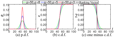
We explore the relationship from the perspective of age label encoding. In DLDL, for a face image x with true age y and hyper-parameter σ, the target vector pld (i.e., label distribution) is generated by a normal p.d.f. (Eq. (1)). For example, the target vector of a 50 years-old face is shown in Fig. 1a. In Ranking CNN, K-1 binary classifiers are required for K age ranks because the k-th binary classifier focuses on determining whether the age rank of an image is greater than lk or not. If y ∈ (lk-1, lk], the target vector with length K-1 is encoded as prank = [1, . . . , 1, 0, . . . , 0], where the first k - 1 values are 1 and the remaining 0. For example, the ranking target vector of a 50 years-old face is shown in Fig. 1c with the dark line.
As we all know, for a generic normal distribution with p.d.f. p, mean y and deviation σ, the cumulative distribution function (c.d.f.) is
where erf(x) = 2 √π ∫ x 0 e-t2 dt. Fig. 1b shows the c.d.f. corresponding to the p.d.f. in Fig. 1a. From Eq. (2), we can easily know
As shown in Fig. 1c, the curve of 1-c is very close to that of prank when σ is set to a small positive real number. Thus, we have
where k = 1, 2, . . . ,K - 1. Eq. (4) shows prank is a specific case of LDL, where the distribution is the cumulative one with σ → 0. That is to say, Ranking is to learn a c.d.f. essentially, while DLDL aims at learning a p.d.f. More generally, we have
where T is a transformation matrix with the form of Tij = 1 for all i ≤ j otherwise 0. Substituting (5) in to (4), we have
Therefore, there is a linear relationship between Ranking encoding and label distribution. The label distribution encoding pld can represent more meaningful age information with different σ, but ranking encoding prank does not. Furthermore, DLDL is more efficient, because only one network has to be trained. However, as discussed earlier, all these methods may be suboptimal because there exists inconsistency between the training objective and evaluation metric.
3.3 Joint Learning for Age Estimation
In order to jointly learn age distribution and output the expectation, in this section we propose the DLDL-v2 framework.
The Label Distribution Learning Module
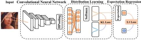
To utilize the good properties of LDL, we integrate it into our framework to formulate an LDL module. As shown in Fig. 2, this module includes a fully connected layer, a softmax layer and a loss layer. This module follows the DLDL method in [Gao et al., 2017].
Specifically, given an input image x and the corresponding label distribution p, we assume that f = F(x; θ) is the activation of the last layer of CNN, where θ denotes the parameters of the CNN. A fully connected layer transfers f to x ∈ RK by
Then, we use a softmax function to turn x into a probability distribution, that is,
Given an input image, the goal of the LDL module is to find θ, W, and b to generate ˆp that is similar to p.
We employ the Kullback-Leibler divergence as the measurement of the dissimilarity between ground-truth label distribution and prediction distribution. Thus, we can define a loss function on one training sample as follows [Gao et al., 2017]:
The Expectation Regression Module
Note that the LDL module only learns a label distribution but cannot regress a precise value. In order to reduce the inconsistency between training and evaluation stages, we propose an expectation regression module to further refine the predicted value. As shown in Fig. 2, this module includes an expectation layer and a loss layer.
The expectation layer takes the predicted distribution and label set as input and outputs its expectation
where ˆ pk denotes the prediction probability that the input image belongs to label lk. Given an input image, the expectation regression module minimizes the error between the expected value ˆ y and ground-truth y. We use ℓ1 loss as the error measurement as follows:
where | · | denotes absolute value. Note that this module does not introduce any new parameter.
Learning
Given a training data set D, the learning goal of our framework is to find θ, W and b via jointly learning label distribution and expectation regression. Thus, our final loss function is a weighted combination of the label distribution loss Lld and the expectation regression loss Ler.
where λ is a weight which balances the importance between two types of losses. Substituting Eq. (9), Eq. (10) and Eq. (11) into Eq. (12), we have
In our framework, optimization variables include W, b and θ. We adopt stochastic gradient descent algorithms of back propagation to optimize them to train our model. The derivative of L with respect to ˆ pk is
For any k and j, the derivative of softmax (Eq. (8)) is well known, as
where δ(k=j) is 1 if k = j, and 0 otherwise. Then,
Applying the chain rule for Eq. (7) again, the derivative of L with respect toW, b and θ are easily obtained
OnceW, b and θ are learned, the prediction value ˆ y of any new instance x is generated by Eq. (10) in a forward network computation.
3.4 Network Architecture
Considering model size and efficiency, we modify the VGG16 architecture [Simonyan and Zisserman, 2015] from four aspects. First, the three fully connected (FC) layers roughly contain 90% parameters of the whole model. We remove all FC layers instead of a hybrid-pooling (HP) which is constructed by a max-pooling (MP) and a global avg-pooling (GAP). Second, to further reduce model size, we reduce the number of the filters in each Conv layer to make it thinner. Third, we add a batch normalization (BN) [Ioffe and Szegedy, 2015] layer after each Conv layer to speed up training. At last, we add label distribution learning module and expectation regression module after the HP, as shown in Fig. 2.
Since we design the network for age estimation and its architecture is thiner than the original VGG16, we call it ThinAgeNet which employs the compression rate of 0.5. 1 We also train a very small model with the compression rate of 0.25, and we call it TinyAgeNet.
4 Experiments
In this section, we conduct experiments to validate the effectiveness of the proposed DLDL-v2 on three benchmark age datasets, based on the open source framework Torch7. All experiments are conducted on an NVIDIA M40 GPU. 2
4.1 Datasets
Two types of age datasets are used in our experiments. The first type contains two small-scale apparent age datasets which are collected in the wild. The second type is a large-scale real age dataset.
ChaLearn15 is from the first competition track ChaLearn LAP 2015 [Escalera et al., 2015]. The dataset has 4699 images and is split into 2476 training, 1136 validation and 1087 testing images. For each image, its mean age and the corresponding standard deviation are given. Since the ground-truth for testing images are not released, we follow the protocol from [Rothe et al., 2018; Gao et al., 2017] to train on the training set and evaluate on the validation set.
ChaLearn16 [Escalera et al., 2016] is an extension of ChaLearn15. It contains 7591 images labeled with apparent age and standard deviation. They are divided into three subsets, including 4113 training, 1500 validation and 1978 testing images. We train the model on training and validation sets and report results on the testing set.
Morph is the largest publicly available real age dataset [Ricanek and Tesafaye, 2006]. There are 55134 face images from more than 13000 subjects. Following the experimental setting in [Niu et al., 2016], we randomly divide the whole dataset into two parts, 80% of the whole dataset for training and the remain 20% for testing.
4.2 EvaluationMetrics
MAE metric is used to evaluate the performance of age estimation. It is the average difference between the predicted and the real age: 1N ∑Nn=1 |ˆ yn - yn |, where ˆ yn and yn are the estimated and the ground-truth age of the n-th testing image, respectively. In addition, a special measurement (ϵerror) is defined by the ChaLearn competition, computed as 1N ∑Nn=1 (1 - exp (- (ˆ yn-yn )2 2(σn )2 )), where σn is the standard deviation of the n-th testing image.
1 0.5 compression rate means every Conv layer has only 50% channels as that in VGG16.
2 Code and pre-trained models will be available at http:// lamda.nju.edu.cn/gaobb/Projects/DLDL-v2.html.
4.3 Implementation Details
Pre-preprocessing We firstly use multi-task cascaded CNN to conduct face and facial points detection for all images [Zhang et al., 2016]. Then, based on these facial points, we align faces to the upright pose. Finally, all faces are cropped and resized to 224×224. Before feeding to the network, all resized images are to subtract mean and divide standard deviation for each color channel.
Data Augmentation There are many non-controlled environmental factors such as face position, illumination, diverse backgrounds, image color and image quality, especially in ChaLearn datasets. To handle these issues, we apply data augmentation techniques, including random horizontal flipping, random scaling, random color/gray changing, random rotation and standard color jittering, to every training image, so that the network can take a different variation of the original image as input at each epoch of training.
Training Details ThinAgeNet/TinyAgeNet is pre-trained by softmax loss on a subset of the MS-Celeb-1M dataset [Guo et al., 2016]. To avoid the imbalance problem among identities, we cut those identities whose number of images is lower than a threshold. In our experiments, we use about 5M images of 54K identities as training data.
After pre-training is finished, we remove classification layer of the network and add the age estimation modules. Then, fine-tuning is conducted on age datasets. All networks are optimized by Adam [Kingma and Ba, 2015], with β1 = 0.9, β2 = 0.999 and ϵ = 10-8 . The initial learning rate is 0.001, and it is decreased by a factor of 10 every 30 epochs. Each model is trained 60 epochs using mini-batches of 128.
Inference Details At the test time, we feed the test image and its flipped copy into the network and average their predictions as the final age estimation.
4.4 Comparisons with State-of-the-Arts
Table 1 reports the comparisons of our method and previous state-of-the-arts on three age estimation datasets.
Low Error In the ChaLearn15 challenge, the best result came from DEX. Its success mainly used a lot of (260,282) external age labeled training images. Under the same setting, our method outperforms DEX by a large margin in Table 3. On ChaLearn16, the ϵ-error 0.267 of our approach is close to the best competition result 0.241 (LDAE). Note that our result is only based on a single model without external age labeled data. LDAE not only used external age labeled data but also employed multi-model ensemble. On Morph, our method creates a new state-of-the-art 1.969 MAE. To our best knowledge, this is the first time to achieve below two years in MAE.
| Methods | External | ChaLearn15 | ChaLearn16 | Morph | ||
|---|---|---|---|---|---|---|
| Data | MAE | ϵ-error | MAE | ϵ-error | MAE | |
| Human [Han et al., 2015] | × | - | 0.34 | - | - | 6.30 |
| OR-CNN [Niu et al., 2016] | × | - | - | - | - | 3.34 |
| DEX [Rothe et al., 2018] | × √ | 5.369 | 0.456 | - | - | 3.25 |
| DEX [Rothe et al., 2018] | 3.252 | 0.282 | - | - | 2.68 | |
| DLDL [Gao et al., 2017] | × | 3.51 | 0.31 | - | - | 2.42 1 |
| Ranking [Chen et al., 2017] | × √ | - | - | - | - | 2.96 |
| LDAE [Antipov et al., 2017] | - | - | - | 0.241 2 | 2.35 | |
| DLDL-v2 (TinyAgeNet) | × | 3.427 | 0.301 | 3.765 | 0.291 | 2.291 |
| DLDL-v2 (ThinAgeNet) | × | 3.135 | 0.272 | 3.452 | 0.267 | 1.969 |
1 Used 90% of Morph images for training and 10% for evaluation; 2 Used multi-model ensemble;
| Methods | #Param(M) | #Time(ms) |
|---|---|---|
| DEX [Rothe et al., 2018] | 134.6 | 133.30 |
| DLDL [Gao et al., 2017] | 134.6 | 133.30 |
| LDAE [Antipov et al., 2017] | 1480.6 | 1446.30 |
| DLDL-v2 (TinyAgeNet) | 0.9 | 24.26 |
| DLDL-v2 (ThinAgeNet) | 3.7 | 51.05 |
High Efficiency We measure the speed on one M40 GPU with batch size 32 accelerated by cuDNN v5.1. The number of parameters and the computation times of forward running of our approach and some previous methods are reported in Table 2. Since OR-CNN and Ranking have not release pretrained models, we cannot test the running time. LDAE's model size and running time is 11 times of DEX and DLDL since 11 models are used to ensemble. Compared to stateof-the-arts, our DLDL-v2 (ThinAgeNet) achieves the best performance using the single model with 36× fewer parameters and 2.6× reduction in inference time. What is more, our tiny model has 150× fewer parameters and 5.5× speed improvement compared to DLDL, which still achieve better performance.
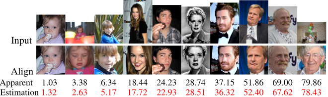
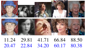
Visual Assessment Fig. 3 shows some examples on ChaLearn16 testing images using our DLDL-v2 with ThinAgeNet. In many cases, our solution is able to predict the age of faces accurately. Failures may come from some special cases such as occlusion, low resolution, heavy makeup and extreme pose.
4.5 Ablation Study
ThinAgeNet is employed for all experiments in this section. We firstly investigate the efficacy of the proposed data augmentation and pooling strategy. For fair comparison, we fix △l = 1 and λ = 1. To investigate the effectiveness of the our proposed joint learning mechanism, we compare it with five very strong methods under the same setting. The comparison results are shown in Table 3.
| Methods | Factors | ChaLearn15 | ChaLearn16 | Morph | |||
|---|---|---|---|---|---|---|---|
| Aug | Pool | MAE | ϵ-error | MAE | ϵ-error | MAE | |
| DLDL-v2 | × √ | HP GAP | 3.399 3.210 | 0.303 | 3.717 | 0.290 | 2.346 2.039 |
| √ | HP | 0.282 0.272 | 3.539 3.452 | 0.274 0.267 | 1.969 | ||
| √ | HP | 3.135 | |||||
| MR (ℓ2) | √ | 3.665 | 0.337 | 3.696 | 0.294 | 2.282 | |
| MR (ℓ1) DEX | √ | HP | 3.655 | 0.334 | 3.722 | 0.301 | 2.347 |
| √ | HP | 3.558 | 0.306 | 4.163 | 0.332 | 2.311 | |
| Ranking | √ | HP | 3.365 | 0.298 | 3.645 | 0.290 | 2.164 |
| DLDL | HP | 3.228 | 0.285 | 3.509 | 0.272 | 2.132 | |
| Hyper-param | ChaLearn15 | ChaLearn16 | Morph | |||
|---|---|---|---|---|---|---|
| λ | △l (K) | MAE | ϵ-error | MAE | ϵ-error | MAE |
| 0.01 | 1 (101) | 3.223 | 0.282 | 3.493 | 0.270 | 1.960 |
| 0.10 | 1 (101) | 3.188 | 0.278 | 3.455 | 0.268 | 1.972 |
| 1.00 | 1 (101) | 3.135 | 0.272 | 3.452 | 0.267 | 1.969 |
| 10.00 | 1 (101) | 3.144 | 0.273 | 3.487 | 0.270 | 1.977 |
| 1.00 | 4 (26) | 3.182 | 0.276 | 3.473 | 0.270 | 1.963 |
| 1.00 | 2 (51) | 3.184 | 0.274 | 3.484 | 0.271 | 1.963 |
| 1.00 | 0.50 (201) | 3.184 | 0.278 | 3.484 | 0.269 | 1.992 |
| 1.00 | 0.25 (401) | 3.167 | 0.274 | 3.459 | 0.265 | 2.028 |
Data Augmentation We can see that about 0.26 and 0.38 MAE improvement on apparent datasets and Morph using data augmentation, respectively. This indicates data augmentation can greatly improve the performance of age estimation.
Pooling Strategy To explore the effect of the pooling strategy, we further use the HP to replace the GAP when combining data augmentation. It can be seen that the proposed HP can consistently reduce the prediction error on all datasets. This indicates that the feature of HP is more discriminative than that of GAP.
Comparisons with Baselines The lower part in Table 3 show the results of all baselines. We can see that the MAE and ϵ-error of Ranking and DLDL methods are significantly lower than that of MR and DEX on all datasets. This indicates that utilizing label distribution is helpful to reduce age estimation error. Meanwhile, we also find that the prediction error of Ranking is close to that of DLDL, which conforms to the analysis in Sec. 3.2. Furthermore, the performance of DLDL is better than that of Ranking, which suggests that learning p.d.f. is more effective than learning c.d.f. The proposed joint learning achieves the best performance among all methods. It means that erasing the inconsistency between training and evaluation stages can help us make a better prediction.
Sensitivity to Hyper-parameters We explore the influence of hyper-parameters λ and △l. In Table 4, we report results on all three datasets with different value of λ and △l. We can see that our methods is not sensitive to λ and △l with 0.01 ≤ λ ≤ 10 and 0.25 ≤ λ ≤ 4.
4.6 HowDoes DLDL-v2 Estimate Facial Age?
To understand how DLDL-v2 makes the final determination, we visualize a score map that can intuitively show which regions of face image are related to the network decision.
Let the last convolution block produce activation maps Fj ∈ Rh′×w′ . These activations are then spatially pooled by a hybrid pooling and linearly transformed (i.e., Eq. (7)) to produce age probabilities ˆ p ∈ RK with a label distribution module. To produce age activation map, we apply linearly transform layer to Fj , i.e. Ak = ∑j wkjFj + bk. Then, the score map can be derived by S = ∑k ˆ pkAk . The value of Sij represents the contribution of the network's decision at position of i-th row and j-th column. Bigger values mean more contributions and vice versa. For comparing the correspondence between highlighted regions in S and an input image, we scale S to the size of input image.
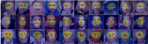
In Fig. 4, we show some examples coming from different age group. we can see that the highlighted regions (i.e., red) are significantly different for different age group faces. For infants, the highlighted region locates in the center of two eyes. For adults, the strong areas include two eyes, nose and mouth. For senior people, the highlighted regions consist of the forehead, brows, eyes and nose. In short, the network uses different patterns to estimate different age.
4.7 Why Does DLDL-v2WorkWell?
Compared to MR, the training procedure of our DLDL-v2 is more stable because it not only regresses the single value with expectation module but also learns a label distribution. Compared to DEX, through introducing label distribution learning module to DLDL-v2, the training instances associated with each class label is significantly increased without actually increasing the number of the total training images, which effectively alleviate the risk of over-fitting. For Ranking and DLDL-based methods, we have shown that they are both leaning a label distribution from different levels. Therefore, they both share the advantages of label distribution learning. However, these methods can not avoid the inconsistency between training objective and evaluation metric. Our proposed DLDLv2 can effectively alleviate this issue. Therefore, it can achieve better performance (Sec. 4.5).
5 Conclusion
In this paper, we firstly analyze that Ranking-based methods are implicitly learning label distribution. This result unifies two existing popular state-of-the-art age estimation methods into the DLDL framework. Second, we propose a DLDL-v2 framework which alleviates the inconsistency between training and evaluation stages via jointly learning age distribution and regressing single age with a thin and deep network architecture. The proposed approach creates new state-of-the-art results on apparent and real age estimation tasks with fewer parameters and faster speed. In addition, our DLDL-v2 is also an interpretable deep framework which employs different patterns to estimate age.
@inproceedings{ijcai2018p99,
  title     = {Age Estimation Using Expectation of Label Distribution Learning},
  author    = {Gao, Bin-Bin and Zhou, Hong-Yu and Wu, Jianxin and Geng, Xin},
  booktitle = {Proceedings of the Twenty-Seventh International Joint Conference on
               Artificial Intelligence, {IJCAI-18}},
  publisher = {International Joint Conferences on Artificial Intelligence Organization},
  editor    = {Jérôme Lang},
  pages     = {712--718},
  year      = {2018},
  month     = {7},
  note      = {Main track},
  doi       = {10.24963/ijcai.2018/99},
  url       = {https://doi.org/10.24963/ijcai.2018/99},
}
TY - CPAPER TI - Age Estimation Using Expectation of Label Distribution Learning AU - Gao, Bin-Bin AU - Zhou, Hong-Yu AU - Wu, Jianxin AU - Geng, Xin T2 - Proceedings of the Twenty-Seventh International Joint Conference on Artificial Intelligence, IJCAI-18 PB - International Joint Conferences on Artificial Intelligence Organization PY - 2018 SP - 712 EP - 718 DO - 10.24963/ijcai.2018/99 UR - https://doi.org/10.24963/ijcai.2018/99 ER -Copied
Machine-readable versions of this paper, for tools and AI agents:





