On the Relation Between Approximation Fixpoint Theory and Justification Theory

1 Introduction

In this framework, we are concerned with two theories developed with similar intentions, namely to unify semantics of (mostly non-monotonic) logics, namely Approximation Fixpoint Theory (AFT) and Justification Theory (JT).

1.1 Approximation Fixpoint Theory

In the 1980s and 90s, the area of non-monotonic reasoning (NMR) saw fierce debates about formal semantics. In several subareas, researchers sought to formalise common-sense intuitions about knowledge of introspective agents. In these areas, appeals to similar intuitions were made, resulting in the development of similar mathematical concepts. Despite the obvious similarity, the precise relation between these concepts remained elusive. AFT was founded in the early 2000s by Denecker, Marek and Truszczy´nski [2000] as a way of unifying semantics that emerged in these different subareas. The main contribution of AFT was to demonstrate that, by moving to an algebraic setting, the common principles behind these concepts can be isolated and studied in a general way.

This breakthrough allowed results that were achieved in the context of one of these languages to be easily transferred to another. In the early stages, AFT was applied to default logic, auto-epistemic logic, and logic programming [Denecker et al., 2000; Denecker et al., 2003]. In recent years also applications in various other domains have emerged [Strass, 2013; Bi et al., 2014; Charalambidis et al., 2018; Bogaerts and Cruz-Filipe, 2018].

The foundations of AFT lie in Tarski's fixpoint theory of monotone operators on a complete lattice [Tarski, 1955]. AFT demonstrates that by moving from the original lattice L to the bilattice L2 , Tarski's theory can be generalised into a fixpoint theory for arbitrary (i.e., also non-monotone) operators. Crucially, all that is required to apply AFT to a formalism and obtain several semantics is to define an appropriate approximating operator L2 → L2 on the bilattice; the algebraic theory of AFT then takes care of the rest. For instance, to characterise the major logic programming semantics using AFT, it suffices to define Fitting's four-valued immediate consequence operator [Fitting, 2002]. The (partial) stable fixpoints of that operator (as defined by AFT) are exactly the partial stable models of the original program; the wellfounded fixpoint of the operator is the well-founded model of the program, etc.

1.2 Justification Theory

Building on an old semantical framework for (abductive) logic programming [Denecker and De Schreye, 1993], Denecker et al. [2015] defined an abstract theory of justifications suitable for describing the semantics of a range of logics in knowledge representation, computational and mathematical logic, including logic programs, argumentation frameworks and nested least and greatest fixpoint definitions. Justifications provide a refined way of describing the semantics of a logic: they not only define whether an interpretation is a model (under a suitable semantics) of a theory, but also why.

Justifications -albeit not always in the exact formal form as described by Denecker et al. [2015] - have appeared in different ways in different areas. The stable semantics for logic programs was defined in terms of justifications [Fages, 1990; Schulz and Toni, 2013]. Moreover, an algebra for combining justifications (for logic programs) was defined by Cabalar et al. [2014]; and justifications are underlying provenance systems in databases [Dam´asio et al., 2013].

Next to these theoretic benefits, justifications are also used in implementations of answer set solvers (they form the basis of the so-called source-pointer approach in the unfounded set algorithm [Gebser et al., 2009], and turned out to be key in analyzing conflicts in the context of lazy grounding [Bogaerts and Weinzierl, 2018]), as well as to improve parity game solvers [Lapauw et al., 2020].

1.3 Correspondence

The two described frameworks were designed with similar intentions in mind, namely to unify different (mainly nonmonotonic) logics. One major difference between them is that JT is defined logically while AFT is defined purely algebraically. This makes justification frameworks less abstract and easier to grasp, but also in a certain sense less general. On the other hand, Denecker et al. [2015] defined a notion of nesting, which seems promising to integrate the semantics of nested least and nested greatest fixpoint definitions.

Despite the differences, certain correspondences between the theories show up: several definitions in justification frameworks seem to have an algebraical counterpart in AFT. This is evident from the fact that many results on justifications are formulated in terms of fixpoints of a so-called derivation operator that happens, for the case of logic programming, to coincide with (Fitting's three-valued version of) the immediate consequence operator for logic programs. Of course, now the question naturally arises whether this correspondence can be made formal, i.e., whether it can formally be shown that semantics induced by JT will always coincide with their equally-named counterpart in AFT. If the answer is positive, this will allow us to translate results between the two theories. Formalising this correspondence is the key contribution of the current paper.

1.4 Contributions

Our contributions can be summarised as follows:

• In Section 3, we provide some novel results for JT. While the main purpose of these results is to support the theorems of Section 4, they also directly advance the state of JT. In this section, we show among others how different semantics induced by JT relate, and we resolve a discrepancy that exists between different definitions of so-called stable and supported branch evaluations in prior work. We formally prove that the different circulating definitions of these branch evaluations indeed induce the same semantics.
• In Section 4, we turn our attention to the key contribution of the paper, namely embedding JT in AFT. To do this, we proceed as follows. First, we show that under minor restrictions, each justification frame (intuitively, this is a set of rules that describe when a positive or negative fact is true), can be transformed into an approximator. Next, we show that for each of the most common branch evaluations (these are mathematical structures that are used to associate semantics to a justification frame), the induced semantics by JT is the same as the equally-named semantics on the AFT
• side. Establishing this result is of particular importance for the future development of JT, since this result immediately makes a large body of theoretical results developed in the context of AFT readily available for JT, as well as all its future application domains, including results on stratification [Vennekens et al., 2006; Bogaerts and Cruz-Filipe, 2021], predicate introduction [Vennekens et al., 2007], and knowledge compilation [Bogaerts and Van den Broeck, 2015]. On the other hand, from the context of AFT, the embedding of JT can serve as inspiration for developing more general algebraic explanation mechanisms.
• To illustrate how this connection can be exploited for further exploiting the theory of justifications, we turn our attention to ultimate semantics. In the context of AFT, Denecker and his coauthors have realised that a single operator can have multiple approximators and that the choice of approximator influences the induced semantics. They also showed that -when staying in the realm of consistent AFT - every operator induces a most precise approximator, and called this the ultimate approximator [Denecker et al., 2004]. In Section 5, we transfer this idea to JT. We show there that by means of a simple transformation 1 on the justification frame, we can obtain ultimate semantics. Importantly, since this transformation is defined independent of the branch evaluation at hand, ultimate semantics are not just induced for the semantics that have a counterpart in AFT, but for all conceivable current and future branch evaluations as well.

2 Preliminaries: Justification Theory

In this section, we use the formalisation of JT as done by Marynissen et al. [2020]. Truth values are denoted t (true), f (false) and u (unknown); we write L for {t, f , u}. We make use of two orders on L, the truth order f ≤t u ≤t t and the precision order u ≤p f, t. JT starts with a set F, referred to as a fact space, such that L ⊆ F; the elements of F are called facts. We assume that F is equipped with an involution ∼: F →F (i.e., a bijection that is its own inverse) such that ∼t = f , ∼u = u, and ∼x ̸= x for all x ̸= u. Moreover, we assume that F \ L is partitioned into two disjoint sets F+ and F- such that x ∈ F+ if and only if ∼x ∈ F- for all x ∈ F \ L. Elements of F+ are called positive and elements of F- are called negative facts. An example of a fact space is the set of literals over a propositional vocabulary Σ extended with L where ∼ maps a literal to its negation. For any set A we define ∼A to be the set of elements of the form ∼a for a ∈ A. We distinguish two types of facts: defined and open facts. The former are accompanied by a set of rules that determine their truth value. The truth value of the latter is not governed by the rule system but comes from an external source or is fixed (as is the case for logical facts).

Definition 1. A justification frame JF is a tuple 〈F,Fd,R〉 such that

1 Essentially, this transformation performs some sort of case splitting.

• Fd is a subset of F closed under ∼, i.e., ∼Fd = Fd; facts in Fd are called defined;
• no logical fact is defined: L∩Fd = ∅;
• R ⊆ Fd ×2F\∅ ;
• for each x ∈ Fd there is at least one element (x,A) ∈ R.

The set Fo of open facts is equal to F \ Fd. An element (x,A) ∈ R is called a rule with head x and body (or case) A. The set of cases of x in JF is denoted JF(x). Rules (x, A) ∈ R are denoted as x ← A and if A = {y1, . . . , yn}, we often write x ← y1, . . . , yn.

Logic programming rules can easily be transfered to rules in a justification frame. However, in logic programming, only rules for positive facts are given; never for negative facts. Hence, in order to apply JT to logic programming, a mechanism for deriving rules for negative literals is needed. For this, a technique called complementation was invented [Denecker et al., 2015]; it is a generic mechanism that allows turning a set of rules for x into a set of rules for ∼x. To define complementation, we first define selection functions for x. A selection function for x is a mapping s: JF(x) → F such that s(A) ∈ A for all rules of the form x ← A. Intuitively, a selection function chooses an element from the body of each rule of x. For a selection function s, the set {s(A) | A ∈ JF(x)} is denoted by Im(s).

Definition 2. For a set of rules R, we define R∗ to be the set of rules of the form ∼x ← ∼Im(s) for x ∈ Fd that has rules in R and s a selection function for x. The complementation of JF is defined as 〈F,Fd,R∪R∗ 〉. A justification frame JF is complementary if it is fixed under complementation, i.e., R ∪ R∗ = R.

Example 1. If R = {x ← a, b; x ← c; }, then R∗ = {∼x ←∼a,∼c; ∼x ←∼b,∼c}.

Definition 3. A directed graph is a pair (N, E) where N is a set of nodes and E ⊆ N ×N is the set of edges. An internal node is a node with outgoing edges. A leaf is a non-internal node.

Definition 4. Let JF = 〈F,Fd,R〉 be a justification frame. A justification J in JF is a directed graph (N,E) such that for every internal node n ∈ N it holds that n ← {m | (n, m) ∈ E} ∈ R;

A justification is locally complete if it has no leaves in Fd. We write J(x) to denote the set of locally complete justifications that have an internal node x.

Example 2. Take Fd = {x,∼x, y,∼y}, Fo = {a,∼a, b,∼b} ∪ L, and R the complementation of {x ← y, a; y ← y, b}, then

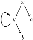
is a locally complete justification in 〈F,Fd,R〉 because a and b are open facts.

Definition 5. Let JF be a justification frame. A JF-branch is either an infinite sequence in Fd or a finite non-empty sequence in Fd followed by an element in Fo. For a justification J in JF, a J-branch starting from x ∈ Fd is a path in J starting from x that is either infinite or ends in a leaf of J. We write BJ(x) to denote the set of J-branches starting from x.

Not all J-branches are JF-branches since they can end in a defined fact. However, if J is locally complete, any J-branch is also a JF-branch. We denote a branch b as b : x0 → x1 → · · · and define ∼b as ∼x0 → ∼x1 → · · · . A tail of a branch b is a branch xi → xi+1 → · · · for some i ≥ 0.

Definition 6. A branch evaluation B is a mapping that maps any JF-branch to an element in F for all justification frames JF. A branch evaluation B is consistent if B(∼b) = ∼B(b) for any branch b. A justification frame JF together with a branch evaluation B form a justification system JS, which is presented as a quadruple 〈F, Fd, R, B〉.

The main branch evaluations we are interested in are given below:

Definition 7. The supported branch evaluation Bsp maps x0 → x1 → · · · to x1. The Kripke-Kleene branch evaluation BKK maps finite branches to their last element and infinite branches to u. The well-founded branch evaluation Bwf maps finite branches to their last element. It maps infinite branches to t if they have a negative tail, to f if they have a positive tail and to u otherwise. The stable branch evaluation Bst maps a branch x0 → x1 → · · · to the first element that has a different sign than x0 if it exists; otherwise b is mapped to Bwf (b).

Definition 8. A (three-valued) interpretation of F is a function I : F → L such that I(∼x) = ∼I(x) for all x ∈ F and I(ℓ) = ℓ for all ℓ ∈ L.

We will assume that the interpretation of open facts is fixed; hence any two interpretations coincide on open facts.

Definition 9. Let JS = 〈F, Fd, R, B〉 be a justification system, I an interpretation of F, and J a locally complete justification in JS. Let x ∈ Fd be a node in J. The value of x ∈ Fd by J under I is defined as valB(J, x, I) = minb∈BJ(x) I(B(b)), where min is with respect to ≤t.

The supported value of x ∈ F in JS under I is defined as SVJS(x, I) = maxJ∈J(x) valB(J, x, I) for x ∈ Fd and SV(x, I) = I(x) for x ∈ Fo. For any F-interpretation I, SJS(I) is the mapping F → L: x ↦→ SVJS(x, I). The function SJS is called the support operator. If JS consists of JF and B, then we write S B JF for SJS. If JF is clear from context, we write SVB for SVJS.

Models under justification semantics are determined by the supported value.

Definition 10. Let JF be justification frame and B a branch evaluation. An F-interpretation I is a B-model of JF if for all x ∈ F, SVBJF (x, I) = I(x), i.e., I is a fixpoint of S B JF .

A Bsp, BKK, Bst, or Bwf -model is called a supported, Kripke-Kleene, stable, or well-founded model.

Example 3. Let F = {p, ∼p, q, ∼q}∪L and take R to be the complementation of {p ← p; p ←∼q; q ← q}, i.e. adding the rules ∼p ← ∼p, q and ∼q ← ∼q. There are exactly two locally complete justifications with p as an internal node:

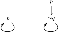
3 Tying Up Loose Ends

In this section, we prove some results about JT that will be needed for developing our theory later on. These results resolve several issues that were left open in prior work, but turn out to be crucial for studying the relationship with AFT.

3.1 Pasting Justifications

Our first result is essentially a pasting result. What it states is that we can, for all branch evaluations of interest to the current paper, build a single justification that explains the value of all facts. In other words, it provides a means of gluing justifications for different facts together. The first theorem has already been proven in a slightly different context by Marynissen et al. [2018].

Theorem 1. Take B ∈ {Bsp, BKK, Bst, Bwf}. For every interpretation I, there is a locally complete justification J such that valB(x, J, I) = SVB(x, I) for all x ∈ Fd.

Similarly, this holds for B′sp and B′st , but only for models.

Theorem 2. Take B ∈ {B′sp , B′st}. For every B-model I, there is a locally complete justification J such that valB(x, J, I) = SVB(x, I) for all x ∈ Fd.

3.2 Equivalence of Branch Evaluations

Our second result concerns different versions of the stable and supported branch evaluations that circulate in prior work. Marynissen et al. [2018; 2020] use the stable and supported branch evaluations as we defined them in Definition 7, while Denecker et al. [2015] use the following alternative.

Definition 11. The branch evaluation B′sp is equal to Bsp on infinite branches and maps finite branches to their last element. The branch evaluation B′st is equal to Bst except B′st maps any finite branch to its last element.

Of course this begs the question in which sense these branch evaluations are related. What we show next is that for the purpose of defining models, they are interchangeable.

Definition 12. Two branch evaluations B1 and B2 are equivalent if for all justification frames JF, the B1-models and the B2-models of JF coincide.

Our proofs that Bsp and B′sp , and Bst and B′st are equivalent, will make use of the following lemma, which intuitively states that to show that an interpretation is a B-model, it suffices to show that the supported value of each fact is at least its value in the interpretation.

Lemma 1. Take JS = 〈F,Fd,R, B〉 with B consistent. Every interpretation I such that SVJS(x, I) ≥t I(x) for all x ∈ Fd, is a B-model of JF.

Proposition 1. The two supported branch evaluations Bsp and B′sp are equivalent.

Proposition 2. The two stable branch evaluations Bst and B′st are equivalent.

Sketch of the proofs of Propositions 1 and 2. The difference between the two branch evaluations at hand is that in the one (B′ ), finite branches are evaluated with respect to their final element, and the other (B) with respect to some other element y in the branch (second or first sign switch). Take a B-model I and take a justification J as from Theorems 1 or 2. With some care, we can prove that the final element of a J-branch has a larger value than first element in I under ≤t. Therefore, I satisfies the conditions of Lemma 1, proving that I is a B′ -model. The other direction is proven similarly.

3.3 Links between Different JustificationModels

Our third set of results is concerned with the relation between different semantics induced by JT. In the context of logic programming, it is well-known that there is a unique wellfounded model, what the relation between well-founded and stable model is, etcetera. Several such results will follow immediately by establishing the correspondence with AFT, but some of them will be needed in our proof. They are given explicitly, and sometimes in higher generality, in the current section.

First of all, in logic programming, it is well-known that the well-founded and Kripke-Kleene semantics induce a single model. In JT, we find an analogous result for a broad class of branch evaluations. A branch evaluation B is called parametric if B(b) ∈ Fo for all JF-branches and all justification frames JF. Denecker et al. [2015] provided the following result.

Proposition 3. If JF is a justification frame and B a parametric branch evaluation, then JF has a single B-model.

In this proposition, we of course make use of our earlier assumption that the value of the open facts is fixed. In general, every interpretation of the open facts induces a single model.

Corollary 1. Every justification frame has a unique BKKmodel and a unique Bwf -model.

Proposition 4. The unique BKK-model is a Bsp-model.

Proposition 5. The well-founded model of JF is a stable model of JF.

Proposition 6. Every stable justification model is a supported justification model.

Proof sketches of Proposition 4, 5 and 6. The idea of the proof is that the justification according to Theorem 1 also works for the other branch evaluation.

Lemma 2. Let I be a stable justification model. If SVBwf (x, I) = f , then I(x) = f . If SVBwf (x, I) = t, then I(x) = t.

Proof sketch. Take x ∈ Fd with I(x) = f . By using that I is a Bst-model, we can prove that every justification J has a branch b ∈ BJ(x) such that I(Bwf(b)) ≤t u. This concludes that SVBwf (x, I) ̸= t.

Proposition 7. The well-foundedmodel is the≤p-least stable model.

Proof sketch. Lemma 2 implies that the well-founded model is less precise than any stable model. Then Proposition 5 finishes the proof.

4 Embedding JT in AFT

We now turn our attention to the main topic of this paper, namely formally prove the correspondence between JT and AFT. We start with a brief recall of the basic definitions that constitute AFT, next show how to obtain an approximator out of a justification frame, and finally prove that indeed, all major semantics are preserved under this correspondence.

4.1 Preliminaries: AFT

Given a complete lattice 〈L, ≤〉, AFT [Denecker et al., 2000] uses the bilattice L2 = L×L. We define projection functions as usual: (x, y)1 = x and (x, y)2 = y. Pairs (x, y) ∈ L2 are used to approximate elements in the interval [x, y] = {z | x ≤ z ≤ y}. We call (x, y) ∈ L2 consistent if x ≤ y, i.e., if [x, y] is not empty. The set of consistent elements is denoted Lc . A pair (x, x) is called exact since it approximates only the element x. The precision order ≤p on L2 is defined as (x, y) ≤p (u, v) if x ≤ u and y ≥ v. If (u, v) is consistent, this means that [u, v] ⊆ [x, y]. If 〈L,≤〉 is a complete lattice, then so is 〈L2 ,≤p 〉. AFT studies fixpoints of operators O: L → L through operators approximating O. An operator A: L2 → L2 is an approximator of O if it is ≤pmonotone and has the property that A(x, x) = (O(x), O(x)) for all x ∈ L. Approximators are internal in Lc (i.e., map Lc into Lc ). We often restrict our attention to symmetric approximators: approximators A such that, for all x and y, A(x, y)1 = A(y, x)2. Denecker et al. [2004] showed that the consistent fixpoints of interest of a symmetric approximator are uniquely determined by an approximator's restriction to Lc and hence, that it usually suffices to define approximators on Lc . Such a restriction is called a consistent approximator. As mentioned before, AFT studies fixpoints of O using fixpoints of A. The main type of fixpoints that concern us are given here.

• A partial supported fixpoint of A is a fixpoint of A.
• The Kripke-Kleene fixpoint of A is the ≤p-least fixpoint of A; it approximates all fixpoints of A.
• A partial stable fixpoint of A is a pair (x, y) such that x = lfp(A(·, y)1) and y = lfp(A(x, ·)2), where A(·, y)1 denotes the function L → L: z ↦→ A(z, y)1 and analogously A(x, ·)2 stands for L→L: z ↦→A(x, z)2.
• The well-founded fixpoint of A is the ≤p-least partial stable fixpoint of A.

4.2 The Approximator

Let JF = 〈F, Fd, R〉 be a justification frame, fixed throughout this section. Our first goal is to define, from a given justification frame, an approximator on a suitable lattice. Following the correspondence with how this is done in logic programming, we will take as lattice the set of exact interpretations (interpretations that map no facts to u except for u itself). It is easy to see that such interpretations correspond directly to subsets of F+. In other words, we will use the lattice 〈L = 2F+ ,⊆〉. Now, the set Lc is isomorphic to the set of three-valued interpretations of F; under this isomorphism, a consistent pair (I, J) ∈ Lc corresponds to the three-valued interpretation I such that for positive facts x ∈ F+, I(x) = t if x ∈ I, I(x) = f if x ̸∈ J, and I(x) = u otherwise.

Definition 13. The operator OJF : L → L of JF maps a subset I of F+ to

The approximator AJF : Lc → Lc of JF is defined as follows

Proposition 8. If no rule body in JF contains u, then AJF is a consistent approximator of OJF .

So far, we are not aware of practical examples with bodies containing u. From now on, we assume that every justification frame does not have u in a rule body. It turns out that in case our justification frame behaves well with respect to negation (if it is complementary), the approximator is the same operator as induced by the branch evaluation Bsp.

Lemma 3. For a complementary justification frame JF, the function AJF and the support operator S Bsp JF are equal.

4.3 Semantic Correspondence

The central result of this section is the following theorem, which essentially states that for all major semantics, the branch evaluation in JT corresponds to the definitions of AFT.

Theorem 3. Take a complementary justification frame JF.

• The partial supported fixpoints of AJF are exactly the supported models of JF.
• The Kripke-Kleene fixpoint of AJF is the unique KripkeKleene model of JF.
• The partial stable fixpoints of AJF are exactly the stable models of JF.
• The well-founded fixpoint of AJF is the unique wellfounded model of JF.

These four points are proven independently; the first follows directly from our observation that AJF and S Bsp JF are in fact the same operator.

Proposition 9. The partial supported fixpoints of AJF are exactly the supported models of JF.

Given the correspondence between supported semantics, the result for Kripke-Kleene semantics follows quite easily.

Proposition 10. The Kripke-Kleene fixpoint of AJF is equal to the unique BKK-model of JF.

Proof sketch. By combining Propositions 4, and 9, we get that the unique BKK-model (denoted here IBKK ) is a fixpoint of AJF. All that is left to show is that it is the least precise one. Assume towards contradiction that this is not the case, i.e., that there is a fixpoint I of AJF such that IBKK ̸≤p I. From this we can find an x ∈ Fd such that either IBKK (x) = f and I(x) = t, or IBKK (x) = f and I(x) = u. In both cases, we have IBKK (x) = f; hence every justification J with x as internal node has a finite branch starting with x mapped to an open fact y with IBKK (y) = f . However, since IBKK and I agree on open facts, this also means that SVB′sp (x, I) = f , contradicting that I is a B′sp -model.

The proof of the third point of Theorem 3 is split in two parts, proven separately in the following propositions.

Proposition 11. Each stable model of JF is a partial stable fixpoint of AJF.

Proof sketch. Take a Bst-model I = (I1, I2) of JF. To show that I is a partial stable fixpoint, we have two lfp equations to prove. We focus on lfp(AJF(·, I2)1) = I1. We know from Theorem 1 that a justification J exists that justifies all facts in I1. Now, this specific justification induces a dependency order on the facts in I1, defined as y ⪯J x if y is reachable in J from x through positive facts. Using the definition of stable branch evaluation, we can see that this order is well-founded and subsequenty prove using well-founded induction on this order that all facts in I1 must be in lfp(AJF(·, I2)1).

For the other direction, we first need the following lemma.

Lemma 4. Let I be a Bsp-model and x ∈ F+ with SVBsp (x, I) = f . It holds that SVBst (x, I) = f .

Proposition 12. Each partial stable fixpoint of AJF is a stable model of JF.

Proof sketch. Let I = (I1, I2) be a partial stable fixpoint of AJF. We prove that SVBst (x, I) = I(x) for x ∈ F+. By consistency of S Bst JF [Marynissen et al., 2018], this proves that I is a stable model of JF. The proof consists of three parts.

The first part is proven by constructing a possibly non-locally complete justification without infinite branches, every internal node positive, and for every node y we have that I(y) = t. The construction is possible because I1 is the least fixpoint of AJF(·, I2)1. The second part is proven similarly. Last part is a consequence of Lemma 4.

Example 4. Let F = {x,∼x, y,∼y, z,∼z} ∪ L and let R be the complementation of {x ← y; y ← ∼z; z ← ∼x, ∼y; }, i.e., it adds the rules ∼x ← ∼y; ∼y ← z; ∼z ← x and ∼z ← y. The approximator AJF has three partial stable fixpoints: ({x, y} , {x, y}), ({z} , {z}) and (∅, {x, y, z}).

Let us take a look at the fixpoint ({x, y} , {x, y}). Since it is a stable fixpoint, we know that ({x, y} , {x, y}) is a least fixpoint of AJF(·, {x, y}). This operator is monotone with respect to ⊆; hence we can construct the fixpoint by iteratively applying the operator on (∅, {x, y}). This produces the following sequence.

The first step uses the rule y ← ∼z, while the second step uses the rule x ← y. Combining the two we get the justifiction x → y → ∼z, which has only true nodes in the model ({x, y} , {x, y}), only positive internal nodes and every defined leaf is negative. This illustrates the first step of the proof of Proposition 12. By extending the found justification, we get a locally complete justification with the same value as the supported value.

The proof of the fourth point of Theorem 3 follows directly from the third point and Proposition 7.

5 Ultimate Semantics for Justification Frames

When applying AFT to new domains, there is not always a clear choice of which approximator to use; the operator on the other hand is often more clear. Denecker et al. [2004] studied the space of approximators and observed that consistent approximators can naturally be ordered according to their precision, where more precise approximator also yield more precise results (e.g., if approximator A is more precise than B, then the A-well-founded fixpoint is guaranteed to be more precise than B's). They also observed that the space of approximators of O has a most precise element, called the ultimate approximator, denoted U(O).

In the context of JT, the justification frame uniquely determines the approximator at hand. Still, we show that it is possible to obtain ultimate semantics here as well. To do so, we will develop a method to transform a justification frame JF into its ultimate frame U(JF). We will then show that the approximator associated to U(JF) is indeed the ultimate approximator of OJF. The result is a generic mechanism to go from any semantics induced by JT (for arbitrary branch evaluations - not just for those that have an AFT counterpart) to an ultimate variant thereof. Our construction is as follows:

Definition 14. Let JF be a complementary justification frame. Let X be the set rules with a positive head. Let X∗ be the least (w.r.t. ⊆) set containing X that is closed under the addition of rules x ← A if there is a rule x ← B with B ⊆ A, or if there are rules x ← {y} ∪A, x ← {∼y} ∪A. Let Y be the complementation of X. Then U(JF) is defined to be the complementary justification frame 〈F, Fd, Y 〉.

Example 5. Let Fd = {x,∼x} and Fo = {a,∼a, b,∼b} ∪ Fo. Take R to be the complementation of {x ← a, x x ← b,∼x}, which adds the following rules

A rule x ← A is minimal, if there is no rule x ← B with B ⊂ A. For determining the supported value, you only need to take minimal rules into account. The justification frame U(JF) has exactly the following minimal rules:

Of course, it contains many non-minimal rules, for example x ← a, b, x.

The justifications in the original system containing x as an internal nodes are exactly the following:

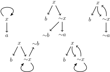
Assume from now on we are working under Bst. The value of the upper left justification for x is f in every interpretation. The values of the other justifications for x are at most u in Bst-models. If it would be t, then the value of these justifications for x is equal to the value of ∼x, which is f .

By taking the ultimate justification frame, the minimal rule x ← a, b is added and the minimal rule ∼x ← x, ∼x is removed. This allows for the justification a ← x → b. If the interpretation of a and b is t, then the value of this justification for x is t. Therefore, ({a, b, x} , {a, b, x}) is an ultimate stable model, while not a stable model. Note that the lower right justification is not a justification in U(JF). If it would be, then this is a true justification for ∼x contradicting the consistency.

It can be seen that the construction adds rules to JF in two cases. For the first type, if x ← B is a rule in R with B ⊆ A, then if B is sufficient to derive x, clearly so is A. The second type of rule addition essentially performs some sort of case splitting. It states that if a set of facts A can be used with either y or ∼y to derive x, then the essence for deriving x is the set A itself. In that case, the rule x ← A is added to the ultimate frame. It turns out that this rule of case splitting is indeed sufficient to reconstruct the ultimate semantics in JT. This is formalised in the main theorem of this section:

An immediate corollary is, for instance that the set of stable models of U(JF) equals the set of ultimate stable fixpoints of OJF, and similarly for other semantics. Recall that, in the context of lattices with the subset order, which is what we are concerned with here, the ultimate approximator is defined as follows [Denecker et al., 2004]:

The proof of Theorem 4 makes use of the following intermediate results.

Lemma 5. Let I be an interpretation and x ∈ Fd. If OJF(I ′ )(x) = t (respectively f) for all exact interpretations I ′ with I ′ ≥p I, then AU(JF)(I)(x) = t (resp. f).

Proof sketch. Take X = {y ∈ Fd | I(x) = u} and let I = (I1, I2). We prove for all Y ⊆ X and all complete consistent sets A over X \ Y that x ← {t} ∪ I1 ∪ ∼(F+ \ I2) ∪ A is a rule in U(JF). If Y = X, then we get that x ← {t} ∪ I1 ∪ ∼(F+ \ I2) is a rule in U(JF) such that its body is true in I, which completes the proof. Our claim is proved by transfinite induction on the size of Y .

Combining this lemma with Eq. (1) of the ultimate approximator immediately yields that the operator AU(JF)(I) is as least as precise as the ultimate approximator of OJF.

Since the ultimate approximator is the most precise approximator of any given operator, all that is left to prove, to indeed obtain Theorem 4 is that AU(JF) indeed approximates OJF. That is the content of the last lemma.

Lemma 7. AU(JF) is an approximator of OJF.

6 Conclusion

In this paper, we presented a general mechanism to translate justification frames into approximating operators and showed that this transformation preserves all semantics the two formalisms have in common. The correspondence we established provides ample opportunity for future work and in fact probably generates more questions than it answers.

By embedding JT in AFT, JT gets access to a rich body of theoretical results developed for AFT, but of course said results are only directly applicable to branch evaluations that have a counterpart in AFT. A question that immediately arises is whether results such as stratification results also apply to other branch evaluations, and which assumptions on branch evaluations would be required for that. Another question that pops up on the JT side is whether concepts such as groundedness [Bogaerts et al., 2015] can be transferred.

On the AFT side, this embedding calls for a general algebraic study of explanations. Indeed, for certain approximators, namely those that "come from" a justification frame, our results give us a method for answering certain why questions in a graph-based manner (with justifications). Lifting this notion of explanation to general approximators would benefit domains of logics that are covered by AFT but not by JT, such as auto-epistemic logic [Moore, 1985] and default logic [Reiter, 1980].

A last question that emerges naturally is how nesting of justification frames, as defined by Denecker et al. [2015] fits into this story, and whether it can give rise to notions of nested operators on the AFT side.

Acknowledgements

Many thanks to Maurice Bruynooghe for the valuable comments and suggestions on draft versions. This research received partial funding from the FWO Flanders project G0B2221N.