
Exploiting Justifications for Lazy Grounding of Answer Set Programs
Proceedings of the Twenty-Seventh International Joint Conference on Artificial Intelligence. Main track. Pages 1737-1745.
https://doi.org/10.24963/ijcai.2018/240
Keywords
- Knowledge Representation and Reasoning: Non-classical Logics for Knowledge Representation
- Knowledge Representation and Reasoning: Non-monotonic Reasoning
- Constraints and SAT: Constraints: Solvers and Tools
Abstract
Answer set programming (ASP) is an established knowledge representation formalism. Lazy grounding avoids the so-called grounding bottleneck of ASP by interleaving grounding and solving; this technique was recently extended to work with conflict-driven clause learning. Unfortunately, it often happens that such a lazy grounding ASP system, at the fixpoint of the evaluation, arrives at an assignment that contains literals that are true but unjustified. The system then is unable to determine the actual causes of the situation and falls back to chronological backtracking, potentially wasting an exponential amount of time.
In this paper, we show how top-down query mechanisms can be used to analyze the situation, learn a new clause or nogood, and backjump further in the search tree. Contributions include a rephrasing of lazy grounding in terms of justifications and algorithms to construct relevant justifications without grounding. Initial experiments indicate that the newly developed techniques indeed allow for an exponential speed-up.
- Krzysztof R. Apt. Principles of Constraint Program- ming. Cambridge University Press, 2003.
- [Balduccini et al., 2013] Marcello Balduccini, Yuliya Lierler, and Peter Schüller. Prolog and ASP inference under one roof. In Proceedings of LPNMR, pages 148-160, 2013.
- [Bichler et al., 2016] Manuel Bichler, Michael Morak, and Stefan Woltran. lpopt: A rule optimization tool for answer set pro- gramming. In Proceedings of LOPSTR, Revised Selected Papers, pages 114-130, 2016.
- [Calimeri et al., 2013] Francesco Calimeri, Wolfgang Faber, Mar- tin Gebser, Giovambattista Ianni, Roland Kaminski, Thomas Krennwallner, Nicola Leone, Francesco Ricca, and Torsten Schaub. ASP-Core-2 input language format. Technical report, ASP Standardization Working Group, 2013.
- [Calimeri et al., 2014] Francesco Calimeri, Giovambattista Ianni, and Francesco Ricca. The third open answer set programming competition. TPLP, 14(1):117-135, 2014.
- [Calimeri et al., 2017] Francesco Calimeri, Davide Fuscà, Simona Perri, and Jessica Zangari. I-DLV: the new intelligent grounder of DLV. Intelligenza Artificiale, 11(1):5-20, 2017.
- [Dal Palù et al., 2009] Alessandro Dal Palù, Agostino Dovier, En- rico Pontelli, and Gianfranco Rossi. GASP: Answer set program- ming with lazy grounding. Fundam. Inform., 96(3):297-322, 2009.
- [Dao-Tran et al., 2012] Minh Dao-Tran, Thomas Eiter, Michael Fink, Gerald Weidinger, and Antonius Weinzierl. Omiga: An open minded grounding on-the-fly answer set solver. In Proceed- ings of JELIA, pages 480-483, 2012.
- [De Cat et al., 2015] Broes De Cat, Marc Denecker, Maurice Bruynooghe, and Peter J. Stuckey. Lazy model expansion: In- terleaving grounding with search. J. Artif. Intell. Res. (JAIR), 52:235-286, 2015.
- [Denecker and De Schreye, 1993] Marc Denecker and Danny De Schreye. Justification semantics: A unifying framework for the semantics of logic programs. In Proceedings of LPNMR, pages 365-379, 1993.
- [Denecker et al., 2015] Marc Denecker, Gerhard Brewka, and Hannes Strass. A formal theory of justifications. In Proceedings of LPNMR, pages 250-264, 2015.
- [Faber et al., 2011] Wolfgang Faber, Gerald Pfeifer, and Nicola Leone. Semantics and complexity of recursive aggregates in an- swer set programming. AIJ, 175(1):278-298, 2011.
- [Gebser et al., 2011] Martin Gebser, Orkunt Sabuncu, and Torsten Schaub. An incremental answer set programming based system for finite model computation. AI Commun., 24(2):195-212, 2011.
- [Gebser et al., 2012] Martin Gebser, Benjamin Kaufmann, and Torsten Schaub. Conflict-driven answer set solving: From the- ory to practice. AIJ, 187:52-89, 2012.
- [Gebser et al., 2015] Martin Gebser, Anna Ryabokon, and Got- tfried Schenner. Combining heuristics for configuration problems using answer set programming. In Proceedings of LPNMR, pages 384-397, 2015.
- [Gebser et al., 2017] Martin Gebser, Marco Maratea, and Francesco Ricca. The sixth answer set programming com- petition. J. Artif. Intell. Res., 60:41-95, 2017.
- [Gelfond and Lifschitz, 1988] Michael Gelfond and Vladimir Lif- schitz. The stable model semantics for logic programming. In Proceedings of ICLP/SLP, pages 1070-1080, 1988.
- [Jansen et al., 2016] Joachim Jansen, Bart Bogaerts, Jo Devriendt, Gerda Janssens, and Marc Denecker. Relevance for SAT(ID). In Proceedings of IJCAI, pages 596-603, 2016.
- [Komorowski, 1992] Henryk Jan Komorowski. An introduction to partial deduction. In Proceedings of META, pages 49-69, 1992.
- [Lefèvre and Nicolas, 2009] Claire Lefèvre and Pascal Nicolas. The first version of a new ASP solver: ASPeRiX. In Proceed- ings of LPNMR, pages 522-527, 2009.
- [Leutgeb and Weinzierl, 2017] Lorenz Leutgeb and Antonius Weinzierl. Techniques for efficient lazy-grounding ASP solving. In Proceedings of Declare 2017, pages 123-138, 2017.
- [Lifschitz, 1999] Vladimir Lifschitz. Answer set planning. In Pro- ceedings of ICLP, pages 23-37, 1999.
- [Marek and Truszczyński, 1999] Victor Marek and Mirosław Truszczyński. Stable models and an alternative logic program- ming paradigm. In The Logic Programming Paradigm: A 25-Year Perspective, pages 375-398. Springer-Verlag, 1999.
- [Marple and Gupta, 2012] Kyle Marple and Gopal Gupta. Galli- wasp: A goal-directed answer set solver. In Proceedings of LOP- STR, Revised Selected Papers, pages 122-136, 2012.
- [Marple et al., 2017] Kyle Marple, Elmer Salazar, and Gopal Gupta. Computing stable models of normal logic programs with- out grounding. CoRR, abs/1709.00501, 2017.
- [Marques-Silva and Sakallah, 1999] João P. Marques-Silva and Karem A. Sakallah. GRASP: A search algorithm for propo- sitional satisfiability. IEEE Transactions on Computers, 48(5):506-521, 1999.
- [Marques Silva et al., 2009] João P. Marques Silva, Inês Lynce, and Sharad Malik. Conflict-driven clause learning SAT solvers. In Armin Biere, Marijn Heule, Hans van Maaren, and Toby Walsh, editors, Handbook of Satisfiability, volume 185 of Frontiers in Artificial Intelligence and Applications, pages 131-153. 2009.
- [Niemelä, 1999] Ilkka Niemelä. Logic programs with stable model semantics as a constraint programming paradigm. Ann. Math. Artif. Intell., 25(3-4):241-273, 1999.
- [Passchyn, 2017] Nico Passchyn. Justification frames. introducing splittable branch evaluations, 2017. Master Thesis;
- [Stuckey, 2010] Peter J. Stuckey. Lazy clause generation: Combin- ing the power of SAT and CP (and mip?) solving. In Proceedings of CPAIOR, pages 5-9, 2010.
- [Taupe et al., 2017] Richard Taupe, Antonius Weinzierl, and Got- tfried Schenner. Introducing Heuristics for Lazy-Grounding ASP Solving. In Proceedings of PAoASP, 2017.
- [Weinzierl, 2017] Antonius Weinzierl. Blending lazy-grounding and CDNL search for answer-set solving. In Proceedings of LP- NMR, pages 191-204, 2017.
- [Zhang et al., 2001] Lintao Zhang, Conor F. Madigan, Matthew W. Moskewicz, and Sharad Malik. Efficient conflict driven learning in Boolean satisfiability solver. In Proceedings of ICCAD, pages 279-285, 2001.
References were extracted automatically from the PDF and may contain errors.
Full text extracted automatically from the PDF; figures, tables and equations may differ. The PDF is the version of record.
1 Introduction
After Gelfond and Lifschitz [1988] defined the stable semantics for logic programs, it was noticed that normal logic programs under this semantics can be used to encode NPhard decision problems [Marek and Truszczy´nski, 1999; Niemel¨a, 1999; Lifschitz, 1999]. This observation started the field of answer set programming (ASP). By now, ASP has matured: ASP users have access to a rich first-order language, ASP-Core2 [Calimeri et al., 2013], to express their knowledge in, and to many efficient ASP solvers [Gebser et al., 2017], building on top of techniques such as conflict-driven clause learning (CDCL) [Marques-Silva and Sakallah, 1999] from satisfiability solving [Marques Silva et al., 2009] and lazy clause generation [Stuckey, 2010] from constraint programming [Apt, 2003].
∗Bart Bogaerts is a postdoctoral fellow of the Research Foundation - Flanders (FWO). Antonius Weinzierl has been supported by the Academy of Finland, project 251170.
To translate ASP-Core2 programs to input for the solvers, first-order variables need to be eliminated by means of grounding. For a long time, progress in ASP mainly focussed on improving efficiency of the solvers, while few grounders were developed. Recently, more attention went to problems where grounding is the bottleneck [Balduccini et al., 2013]. Examples include queries, such as reachability over a large graph; planning problems, with a very large number of potential time steps, or problems where the full grounding contains a lot of unnecessary information and the actual search problem is not very hard. To circumvent the grounding bottleneck, different techniques are being developed. For example, intelligent grounding [Calimeri et al., 2017] and rule decomposition [Bichler et al., 2016] allow to mitigate the grounding bottleneck and for query problems, top down evaluation is often used. For planning instances, and related types of problems incremental grounding [Gebser et al., 2011] is used, for instance, to introduce time steps on-the-fly, when the solver notices no solution exists in the given window. More generally, lazy grounding is a class of techniques that construct parts of the grounding when the solver needs them. Bottom-up lazy grounding systems include Omiga [DaoTran et al., 2012], GASP [Dal Pal`u et al., 2009], ASPeRiX [Lef`evre and Nicolas, 2009] and the recently introduced ALPHA [Weinzierl, 2017] that integrates lazy grounding with a CDCL solver. Also top-down lazy grounding techniques [De Cat et al., 2015] and top-down stable model generation techniques that avoid grounding [Marple and Gupta, 2012; Marple et al., 2017] exist.
In this paper, we focus on ALPHA; more specifically, we provide a solution for one of its weaknesses. ALPHA works by grounding only those rules whose positive body is satisfied (in the assignment maintained by the solver); it might happen that a certain atom, say p, is true due to a constraint, while there are no rules in the grounding that derive p. Consider the following simple example
This program contains a constraint that p must be true, a fact r(17), a rule that derives p if q(17) holds and a choice rule for all q(X) with X ∈ {1..20}. On this example, ALPHA will give rules (1), (2), and (4) to the solver, but the rule (3) will only be given to the solver if it reaches an assignment where q(17) is true. Hence, as soon as the solver chooses q(17) to be false, it loses the possibility to find a stable model. Currently, ALPHA has no mechanism to analyze why rules deriving p are missing. Using top down techniques, we present exactly such a mechanism, that in this case allows ALPHA to back-jump to the decision level where q(17) was decided. Intuitively, our analysis works as follows. We start from an atom for which deriving rules are missing (in our example: p). For each rule that could derive p, it picks an atom from the body of the rule that explains why this rule did not derive p. Whenever possible, it avoids instantiating. In our example, the algorithm would pick q(17) and (r(X),X ̸= 17), where the latter is a symbolic representation of the set of all atoms r(X) with X ̸= 17. Our algorithm then recursively also searches for explanations for those literals. In the current case, q(17) was simply a choice and hence does not need to be explained further and there are no rules that could derive an atom r(X) with X ̸= 17. Hence, the algorithm terminates and returns the explanation that q(17) being false is what causes p to not be derived. In the algorithmwe present, there is some liberty with respect to the order in which literals in a rule body are considered. In our specific example, this could lead, for instance to the algorithm picking q(17) and (q(X), X ̸= 17) as an explanation for the lack of derivations of p. This is much less optimal and would resort to chronological backtracking again. As such, there is a lot of room for heuristics to optimize our algorithm in the future.
We implemented this idea in ALPHA. Preliminary experiments highlight a class of problems where exponential speedups can be achieved.
Our main contributions are: (i) a novel formalization and partial proof of correctness of ALPHA, based on justifications [Denecker et al., 2015], (ii) algorithms to construct justifications in order to learn a new clause that makes ALPHA backjump, and (iii) an extension of ALPHA allowing up to exponential speed up as initial benchmarks show. The ideas and algorithms developed here are not just limited to ALPHA; they are also applicable to other lazy grounding approaches to ASP such as Omiga and ASPeRiX.
2 Preliminaries
Answer Set Programming. Let C be a set of constants, V be a set of variables, and Q be a set of predicates, each with an associated arity, i.e., elements of Q are of the form p/k where p is the predicate name and k its arity. A (non-ground) term is an element of C ∪ V. 1 The set of all terms is denoted T . A (non-ground) atom is an expression of the form p(t1, . . . , tk) where p/k ∈ Q and ti ∈ T for each i. The set of all atoms is denoted A. If p ∈ A, then var(p) denotes the set of variables occurring in p. We say that p is ground if var(p) = ∅. The set of all ground atoms is denoted Agr . A literal is an atom p or its negation ¬p. The former is called a positive literal, the latter a negative literal. Slightly abusing notation, if l is a literal, we use ¬l to denote the literal that is the negation of l, i.e., we use ¬(¬p) to denote p. The set of all literals is denoted L and the set of ground literals Lgr . A clause is a disjunction of literals. A (normal) rule is an expression of the form
1 Following Weinzierl [2017], we omit function symbols to simplify the presentation. All our results still hold in the presence of function symbols, except for termination, for which additional (syntactic) restrictions must be imposed.
where p is an atom and L a set of literals. If r is such a rule, its head, positive body, negative body and body are defined as H(r) = p, B+(r) = A ∩ L, B- = {q ∈ A | ¬q ∈ L} and B(r) = L respectively. We call r a fact if B(r) = ∅ and ground if p and all literals in L are ground. We use var(r) to denote the set of variables occurring in r. A rule r is safe if all variables in r occur in its positive body, i.e., if var(r) ⊆ var(B+(r)). A logic program P is a finite set of safe rules. P is ground if each r ∈ P is. In our examples, logic programs are presented in a more general format, using, e.g., choice rules (see [Calimeri et al., 2013]). These can easily be translated into the format considered here.
A variable substitution is a mapping σ : V → T . We write [t1/X1, . . . , tn/Xn] for the substitution that maps each Xi to ti and each other variable to itself. The result of applying a substitution σ to an expression (term/atom/literal/rule) e is the expression obtained by replacing all variables X by σ(X) and is denoted σ(e). If p and q are two atoms, a substitution σ such that σ(p) = σ(q) is a unifier of p and q. A unifier σ is most general, if for any unifier σ1 there is a substitution σ2 such that σ1 = σ ◦ σ2. We denote the most general unifier of p and q by mgu(p, q). Given two (not necessarily ground) atoms p and q, we say p is an instance of q if there exists a substitution σ such that p = σ(q). Given an expression e, if σ maps var(e) into C, we call σ a grounding substitution (of e). The grounding of a rule is given by
and the (full) grounding of a program P is defined as gr (P) = ⋃r∈P gr (r).
A (Herbrand) interpretation I is a finite set of ground atoms. The satisfaction relation between interpretations and literals is given by I |= p if p ∈ I and I |= ¬p if p ̸∈ I. An interpretation satisfies a set L of literals if it satisfies each literal in L. Given an interpretation I and a ground program P, the FLP-reduct [Faber et al., 2011] of P with respect to I, is P I = {r | I |= B(r)}. An interpretation I is a model of a ground program P if for each rule r ∈ P with I |= B(r), also I |= H(r). An interpretation I is a stable model (or answer set) of a ground program P [Gelfond and Lifschitz, 1988] if it is a subset-minimal model of P I . If P is non-ground, we say that I is an answer set of P if it is an answer set of gr(P). The set of all answer sets of P is denoted AS(P).
A partial interpretation is a consistent set (does not contain both p and ¬p) of ground literals. The value of a literal l in a partial interpretation I is lI = t if l ∈ I, f if ¬l ∈ I and u otherwise.
Justifications. We briefly provide some background on justifications [Denecker et al., 2015; Denecker and De Schreye, 1993; Passchyn, 2017]. Our presentation is limited: we do not cover the entire theory, but a version specialized for ASP, i.e., by only considering the stable branch evaluation. In this section, assume P is a ground logic program. A P-justification J with domain DJ ⊆ Lgr is a function DJ → 2Lgr such that
- For each positive literal p ∈ DJ, there is a rule p ← S in P such that S ⊆ J(p).
- For each negative literal ¬p ∈ DJ and rule p ← S in P, it holds that ¬S ∩J(¬p) ̸= ∅, with ¬S = {¬s | s ∈ S}.
A justification explains for the literals it its domain why they are true. For atoms, this explanation is a rule that derives it, for negative literal, it is a witness that no rule can derive its underlying atom (a set that contains at least the negation of one literal in every rule that could derive that atom). Of course, not every justification provides a sensible reason why something is true, as illustrated below.
Example 2.1. Let P denote the logic program {p ← p.} The function p ↦→ {p} is a justification, depicted 2 below
It is clear that in the unique stable model of P, p is false. Hence, any explanation why it is true should be rejected. ▲
A justification J is locally complete if J(DJ) ⊆ DJ, i.e., if every literal that is used as the explanation of another literal is itself explained. A branch in a locally complete justification is a sequence (li)i∈[0..n] or (li)i∈N such that for each i, li+1 ∈ J(li). A branch is positive if all its literals are positive, negative if all its literals are negative and mixed otherwise. If B = (li) is a mixed branch, we denote by ch(B) the first literal with a sign switch, i.e., its first negative literal if l0 is positive and the first positive literal otherwise. A branch is maximal if it cannot be extended to a longer branch. The value of a branch B of a locally complete justification J in a partial interpretation I, denoted ν(B, I) is a truth value (t, f or u) defined as follows
- ν(B, I) = ch(B)I if B is mixed,
- ν(B, I) = lIn if B = (li)i∈[0..n] and B is not mixed,
- ν(B, I) = f if B is an infinite positive branch,
- ν(B, I) = t if B is an infinite negative branch.
The truth values are ordered in the truth order f ≤t u ≤t t. The value ν(J, I) of a locally complete justification J is defined as the ≤t-minimal value of its maximal branches. The value of a justification J (not neccesarily locally complete) in I is t (respectively f) if all locally complete extensions of J have value t (resp. f ) in I, and u otherwise. A justification J justifies a literal l in I if l ∈ DJ and ν(J, I) = t. We say l is justified by P if there exists a P-justification that justifies l.
Example 2.2. Consider the following program
And consider the interpretations I1 = {p, r} and I2 = {p, s}. The former is a stable model of P, the latter is not. The following justification J1 justifies p, r, ¬q and ¬s in I1.
2 We often depict a justification J as a directed graph G = (V, E) with V = DJ ∪ J(DJ) and (l, l′ ) ∈ E if and only if l′ ∈ J(l).
There exists no justification that justifies ¬r in I2. In fact, the following is a justification that justifies r in I2:
The existence of such a justification means that ¬r cannot be justified in I2. ▲
The following proposition explicates the link between stable models and justifications. It is due to Denecker et al. [2015] (Theorem 1).
Proposition 2.3. The following statements are equivalent:
- I is a stable model of P,
- I is a model of P and for each p ∈ A with I |= p, there exists a justification that justifies p in I.
3 ALPHA and Justifications
The ALPHA algorithm. We present a new formalization of the ALPHA algorithm [Weinzierl, 2017]. Our presentation differs from the original, as we rephrase conditions in terms of justifications. One terminological differences worth pointing out is that we do not use truth values MUST-BETRUE, TRUE, FALSE and UNASSIGNED, but instead keep track of the truth of atoms and whether or not they are justified. For instance, the truth value MUST-BE-TRUE from Weinzierl [2017] corresponds to t but not justified in our setting, while TRUE from Weinzierl [2017] corresponds to t and justified in our setting. The state of ALPHA is a tuple 〈P, Pg , C, α, SJ 〉, where
- P is a logic program,
- Pg ⊆ gr(P) is the so-far grounded program; we use Σg ⊆ Agr to denote the set of ground atoms that occur in Pg ,
- C is a set of (learned) clauses,
- α is the trail; this is a sequence of tuples (l, c) with l a literal and c either the symbol δ, a rule in Pg or a clause in C. α is restricted to not containing no two tuples (l, c) and (¬l, c′ ); in a tuple (l, c) ∈ α, c represents the reason for making l true: either decision (denoted δ) or propagation because of some rule or clause; α implicitly determines a partial interpretation denoted Iα = {l | (l, c) ∈ α for some c}.
- SJ ⊆ A is the set of atoms that are justified by Pg in Iα.
For clause learning and propagation, a rule p ← L is treated as the clause ¬p ∨ ∨l∈L l. Whenever we refer to "a clause" in the following, we mean any rule in Pg (viewed as a clause) or clause in C. We refer to rules whenever the rule structure is needed (for determining justified atoms).
ALPHA interleaves CDCL and grounding. It performs (iteratively) the following steps (listed by priority).
conflict If a clause in C ∪ Pg is violated, analyze the conflict, learn a new clause (add to C) and back-jump (undo changes to α and SJ that happened since a certain point) following the so-called 1UIP schema [Zhang et al., 2001].
(unit) propagate If all literals of a clause c ∈ C∪Pg except for l are false in Iα, add (l, c) to α.
justify If there is a rule r such that B+(r) ⊆ SJ and ¬B-(r) ⊆ Iα, add H(r) to SJ .
ground If, for some grounding substitution σ and r ∈ P, B+(σ(r)) ⊆ Iα, add σ(r) to Pg.
- decide Pick (using some heuristics [Taupe et al., 2017]) one atom p, occurring in Pg that is unknown in Iα and add (p, δ) or (¬p, δ) to α. 3
- justification-conflict If all atoms in Pg are assigned while some atom is true but not justified, learn a new clause, namely ¬l1 ∨ · · · ∨¬ln where the li are all the decisions in α and backtrack (undo changes to α and SJ that happened in the last decision level).
Motivation. One of the weak points of ALPHA is the step justification-conflict. This step is used when the solver arrives in a state where an atom is true but not justified and none of the other rules apply. Intuitively, this means that due to choices of the solver, there are not enough rules to derive this atom (or one of the atoms it depends on), either because the grounder did not produce them, or because certain decisions imply a rule does not fire. In that case, ALPHA resorts to chronological backtracking. This is not optimal as the reason why an atom is unjustified might only be related to certain choices. To illustrate this, consider the following example.
Example 3.1. Let P denote the following program.
When given this program, ALPHA starts by adding rules (5), (8) and all ground instances of rules (6) to Pg. Next, it propagates p(e) to be t. Next, it makes a choice on one of the atoms of q, say it chooses q(e) false, and subsequently all other qs false too. Now, no rules but justification-conflict apply. The atom p(e) is true but not justified. As can be seen, the reason why p(e) is unjustified is the fact that no single rule with p(e) in the head was grounded, which in turn is explained by the fact that q(e) was chosen false. Instead of backtracking, the reasonable option here would be to undo all choices (backtrack to level 0) and learn the clause q(e).
In the terminology of justifications, ¬p(e) is justified by gr(P) in Iα as witnessed by the following justification
The black part of this justification represents the relevant information, i.e., that the choice to make q(e) false blocks all possibilities to justify p(e). ▲
Lazy Grounding and Justifications. We now formally prove our observation from the previous section. More concretely, we show that whenever the rule justification-conflict is used for p, ¬p is justified. From this, it follows that there is no answer set that extends the current assignment. Hence, we can conclude that backtracking is indeed correct whenever such a state is found. The proof of our main result is constructive and hence yields a way to actually build a justification for ¬p. Such a justification provides valuable information: it highlights parts of the current assignment responsible for ¬p being justified. As such, by analyzing it, we can devise a smarter back-jumping mechanism for justificationconflict. In practice, however, this result not directly usable, as it makes use of the full grounding of P. In the next section, we provide an algorithm that builds such a justification without constructing gr(P).
3 ALPHA actually only allows deciding on certain atoms, hence our presentation is slightly more general.
Theorem 3.2. Assume ALPHA is in a state 〈P, Pg, C, α, SJ〉 where no rules but justification-conflict apply. If p is true but not justified by Pg in Iα, then ¬p is justified by gr(P) in Iα.
The proof is omitted due to page restrictions. The idea is that using the fact that ALPHA did not ground certain rules, we can construct a justification for rules in gr(P) \ Pg (if ALPHA did not ground a rule, at least one positive literal in its body is not true and hence, not justified) and using the fact that p is not justified by Pg, we can construct a justification of ¬p in Pg. With some caution, they can be "glued together".
4 Analyzing Unjustifiedness
In the previous section, we showed that whenever the solver arrives in a state where all atoms in Σg have been decided and p is true but not justified, there exists a justification J of ¬p by gr(P) such that ν(J, Iα) = t. This justification explains why p is not justified. However, this is a justification by gr(P), which we do not wish to construct (avoiding this is why we apply lazy grounding in the first place). The algorithm we present below avoids the grounding phase, taking inspiration from top-down logic programming techniques. In a nutshell, the algorithm performs a form of partial deduction (also known as partial evaluation) [Komorowski, 1992], starting from the atom that is true but unjustified and iteratively unfolding rules. What we add are (i) a loop-breaking mechanism for stable semantics, (ii) a way to take the current interpretation of the solver into account, and (iii) a way to keep track of which substitutions of each rule are relevant.
The idea underlying the algorithm is that instead of building a justification where nodes are ground literals, we build a justification where nodes are sets of ground literals (represented symbolically using non-ground literals); the special case where such a such a set is a singleton corresponds to a justification. Such a set, called litset below, represents ground literals that need to be justified without explicitly enumerating all those ground literals. Before providing formal definitions, we illustrate this idea in a small example.
Example 4.1. Let P denote the following logic program.
Consider an interpretation where all atoms over s are false while r, t(1), t(2), and t(3) are true. In this case, r is true but not justified. The following graph:
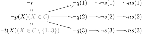
describes (symbolically) why ¬r is justified without actually computing the entire grounding of P. What it represents is:
- ¬r is justified because of a lack of constants c such that p(c) holds.
- The lack of such constants is explained by t not being true outside {1..3}, and q not being true in {1..3}
It can be seen as a first-order representation of the justification
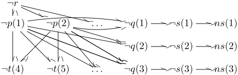
This justification is far from minimal. For instance ¬q(2) is not required to explain ¬p(1). However, it is a good justification of ¬r that is true in every partial interpretation where s(1), s(2) and s(3) are false. Without constructing it, from the first-order representation, we conclude that a reason for r not being justified is that s(1), s(2) and s(3) are false. ▲
Definition 4.2. A litset is a tuple (l, N) where l is a (possibly non-ground) literal and N is a set of substitutions of variables occurring in l.
The litset (l,N) is a first-order representation of the set
We say that a (non-ground) literal q is covered by a litset (p, N) if each ground instance of q is an element of set(p, N).
The intuition behind our algorithm is as follows. We start from a ground literal ¬p such that p is true but unjustified. This literal is represented by the litset (¬p, ∅). During a run, we construct a graph of litsets as a compact, first-order representation of a justification. The graph is constructed in such a way that the corresponding justification evaluates to true in Iα: the domain of the justification consists only of negative literals and the leafs of the justification (elements occurring in the justification but not in the domain) are true positive literals. As such, all branches of the justification are: either mixed and ending in a true literal or infinite and negative. To construct it, we keep track of:
- A set D (for "done") of litsets that are already explained,
- A set TD (for "todo") of litsets that still need to be explained in terms of atoms known to the solver,
- A set L (for "leafs") of ground literals that form the leafs of the justification.
Input: A true, but unjustified atom p, a set of justified atoms SJ and a partial interpretation Iα Output: A set of ground literals L s.t. in each interpretation that contains L, p is true but unjustified 1 L,D,TD← {p}, ∅, {(¬p, ∅)} 2 while TD ̸= ∅ do 3 Pick x ∈ TD 4 (TD′ , L′ ) ← EXPLAINUNJUST(x, SJ , Iα) 5 D←D∪ {x} 6 (TD, L) ← ((TD ∪ TD′ ) \ D, L ∪ L′ ) 7 return LAlgorithm 2: EXPLAINUNJUST: Find a set of litsets that covers all bodies of rules with head p.
Input: A litset (¬p,N) such that all literals in set(p,N) are unjustified, a set of justified atoms SJ , and a partial interpretation Iα
Output: A set of litsets TD′ and a set of ground literals
L′ 1 L′ ,TD′ ← ∅, ∅ 2 foreach rule r ∈ P s.t. σ =mgu(H(r), p) exists do 3 if ∃σN ∈ N s.t. σN(p) is an instance of σ(p) then 4 continue 5 N′ ←N 6 foreach literal lg ∈ Iα, lb ∈ σ(B-(r)) with mgu(lg, lb) = σgb do 7 if ¬∃σN ∈ N s.t. σN(p) is an instance of σgb(σ(p)) then 8 N′ , L′ ← N′ ∪ {σgb ◦ σ}, L′ ∪ {lg} 9 TD′ ←TD′∪UNJUSTCOVER(B+(r), {σ},N′ , SJ) 10 return TD′ ,L′It is an invariant of the algorithm that the sets TD and D only consist of negative literals (¬p, N) such that set(p, N) is a set of atoms not justified by Pg. The algorithm iteratively picks one literal from TD. For that literal, it iterates over all rules of which the head unifies with this literal. For each such rule, and each grounding substitution of that rule, it picks at least one literal and adds its negation either to L or to TD. In order to pick literals, the following priorities are followed:
- P1 If a negative literal in the body of the rule is false, add the negation of such a literal to L, since there is no need for further explanation of such literals.
- P2 For the cases not covered by the above, add the negation of some unjustified positive literal in the body of the rule.
Whenever possible, instead of resorting to actual ground literals, we use litsets, to avoid instantiating too much.
The complete algorithm is described as Algorithms 1, 2, and 3. In the algorithms, whenever we compute a most general unifier, we assume variables have been renamed so that the two literals involved do not share any variables. Algo-
Algorithm 3: UNJUSTCOVER
Input: A set of positive literals B, two sets of variable substitutions Y and N and a set of justified literals SJ Output: A set of litsets such that all their instances are unjustified, and such that for each relevant instance of B (those obtainable after applying a substitution in Y but not by one in N), at least one literal is covered by the result. 1 if B = ∅ or Y = ∅ then return ∅ 2 Pick b ∈ B 3 TD← ∅ 4 foreach σy ∈ Y do 5 Y ′ ← {σ ∣∣∣ σ(b) ∈ SJ ∧ σ(b) instance of σy(b)∧ ¬∃σn ∈ N s.t. σ(b) instance of σn(b) } 6 TD←TD∪ {(σy(b), Y ′ ∪N)} ∪ UNJUSTCOVER(B \ {b}, Y ′ , N, SJ ) 7 return TDrithm 1 specifies the main control: it keeps track of the sets sets D and TD as well as the collection of leaves L found so far. It iteratively picks a litset fromTD, calls Algorithm 2 on it and moves it to D (lines 4 and 5); the results of the call to Algorithm 2 are then added to TD and L (line 6), with the exception of litsets that are already explained: elements of D are never added to TD again. By not adding them again, loops are broken: the same litset can only be explained once. This loop breaking is consistent with stable semantics as the justification we are (implicitly) constructing only has negative literals in its domain.
Algorithm 2 explains why there are no more justified instances of its input litset. For this, it iterates over all rules that could derive the atom of the given litset (lines 2 - 9). For each rule it first checks if the unifier required to derive the current head is excluded by the set N and then skips the rule (lines 3 and 4). Second, N is copied in order to have one version per rule r. Then it implements above priority P1 (in the loop on lines 6 - 8) as follows: it searches the current interpretation Iα for falsified instances of negative literals of the body of r (line 6), and if they are not already excluded by N (line 7), adds them to the set of leafs L′ and excludes the corresponding substitutions from being considered subsequently by adding them to N′ (line 8). Finally, Algorithm 3 is invoked to deal with all cases not covered yet (line 9).
Algorithm 3 implements above priority P2 by searching positive unjustified literals in the rule body for all substitutions not excluded by the previous cases. For this, it picks a literal in the positive body of the rule (line 2) and loops over all substitutions to be handled (lines 4 - 6). There it splits into two cases: (i) for all substitutions yielding justified instances of that literal, it must pick another literal from the positive body; (ii) all other substitutions yield positive unjustified literals. Those substitutions that yield justified literals that are not excluded by N are collected in Y ′ (line 5). This is used in the recursive call to UNJUSTCOVER that finds literals in the rest of the body (for substitutions from (i)) as well as to form the litset (σY (b), Y ′ ∪ N) representing all unjustified literals of case (ii) (all in line 6). Finally, the union of all litsets found in this and the recursive call is returned (line 7).
Theorem 4.3 shows how this algorithm can be used. It provides a clause that can be learned from a call to ANALYZE and shows that learning that clauses advances the solver and that learning it is indeed correct.
Theorem 4.3. Assume an atom p, a set of atoms SJ and a partial interpretation I are given such that
- SJ is the set of atoms justified by P in I,
- p ̸∈ SJ and pI = t,
- for each rule r ∈ P and each grounding substitution σ, if σ(B+(r)) consists of only atoms true in I, then all atoms occurring in σ(r) are assigned a value in I.
Let L = ANALYZE(p, SJ , I) and let c denote the clause ¬p∨ ∨l∈L l. The following claims hold:
- The clause c is violated in I.
- The clause c holds in every answer set of P.
Sketch of the proof. The fact that c is violated follows by construction: only false literals are added to L and p is true in I.
By recording calls to EXPLAINUNJUST, we construct a graph of ground literals. We show that this graph is a justification of ¬p by gr(P). The resulting justification has a negative domain and only positive leafs. Hence, it evaluates to true in each interpretation where its leafs hold. In particular this means that p must be false in each stable model in which the leafs of the justification are true. Hence, c holds in each answer set of P.
Example 4.4 (Example 4.1 continued). Consider again the interpretation I where all atoms over s are false while r, t(1), t(2), and t(3) are true. Let SJ denote {t(1), t(2), t(3)}. Assume ANALYZE(r, SJ, I) is called. First, this algorithm will call EXPLAINUNJUST((¬r, ∅), SJ, I), which returns the explanation (¬p(X), ∅) to be added to TD. Subsequently, the call to EXPLAINUNJUST((¬p(X), ∅), SJ, I) returns TD′ = (¬t(X), {[1/X], [2/X], [3/X]}), (¬q(1), ∅), (¬q(2), ∅), (¬q(3), ∅). The algorithm continues by adding these to TD and calling EXPLAINUNJUST on each of them until TD is empty. As can be seen: the arrows in the first graph in Example 4.1 correspond exactly to the return patterns of calls to EXPLAINUNJUST. ▲
5 Evaluation
We implemented the justification analysis in ALPHA 4 and present the results of our experiments. The benchmarks were run on a cluster of Linux machines with Intel Xeon E5-2680 v3 CPUs. Each benchmark was given 300 seconds and 8GB of memory on a single core of the cluster. Every run requested 10 answer sets and if a problem admits random instances, the reported run times are an average over 10 different random inputs while for other problems it is the average over 5 runs on the same instance. We use ALPHA to refer to the solver without our modifications and ALPHAJ for our extended version. For reference, we also show run times of CLINGO. Our hypothesis is that on problems where justification-conflict occurs, exponential speed-ups can be achieved by ALPHAJ in comparison to ALPHA. We test this on four problem classes, where the first two are synthetic problems, the third is graph colorability, and the fourth is a problem inspired by combined configuration problems [Gebser et al., 2015]. Grounding is an issue only for the last problem, hence it is to be expected that CLINGO performs significantly better than ALPHA or ALPHAJ on the first three (easy-to-ground) problems. The instances used for benchmarking are available at https:// dtai.cs.kuleuven.be/krr/experiments/alpha justifications.zip.
4 ALPHA is freely available at: https://github.com/alpha-asp/ Alpha
Two-way-derivation. The first synthetic problem designed to trigger justification-conflict selects an interpretation for a unary predicate q and then derives atoms over p via two ways; either directly or via an intermediate predicate r. Finally, it enforces that p(5) and p(7) must hold.
Since there are two possible ways to derive p(5) and p(7), the explanation is simple but not trivial. The results are shown in Table 1, where ALPHA hits the timeout already at a domain of size 30 while ALPHAJ only needs 1.56 seconds for a domain even of size 1000. For CLINGO the same problem is trivial, since the program is easy to ground and once the full grounding is available, all rules deriving p(5) and p(7) are known and tailored techniques to keep track of justifications, such as completion no-goods and source pointers [Gebser et al., 2012], can be employed.
Variable-projection. The second synthetic problem selects an interpretation for a binary predicate q over a domain dom, then derives atoms over a unary predicate p and finally enforces that p(5) and p(7) hold.
The rule that derives p projects the variable Y away; hence, there are multiple options to derive for instance p(5). As such, the explanation of why it is not derived is non-trivial. The results are given in Table 2. Without justifications analysis, ALPHA hits the timeout even at size 20 while the time for ALPHAJ increases at a much slower pace and seems in line with the expected quadratic growth of the q predicate. For CLINGO, only the biggest instances require noticeably time. We suspect the difference between CLINGO and ALPHAJ to be mainly caused by CLINGO employing sophisticated rule instantiation techniques while ALPHAJ still uses a semi-naive instantiation mechanism.
Graph-5-coloring. The third benchmark is the well-known graph coloring problem from the ASP competition [Calimeri et al., 2014], which was previously used by Leutgeb and Weinzierl [2017] to benchmark ALPHA. The original encoding of the ASP competition contains for each node n an atom colored(n) defined to be true when n is assigned at least one color. Furthermore, it contains the constraint that each of these atoms must be true. Such a constraint is prone to trigger justification-conflict. However, in the experiments by Leutgeb andWeinzierl [2017], the following redundant constraint was added 5 :
| Size | ALPHA | ALPHAJ | CLINGO |
|---|---|---|---|
| 10 | 0.81 | 0.79 | 0.00 |
| 20 | 2.55 | 0.81 | 0.00 |
| 30 | 300.00(5) | 0.85 | 0.00 |
| 40 | 300.00(5) | 0.92 | 0.00 |
| 50 | 300.00(5) | 0.90 | 0.00 |
| 65 | 300.00(5) | 0.86 | 0.00 |
| 100 | 300.00(5) | 1.02 | 0.00 |
| 200 | 300.00(5) | 1.04 | 0.01 |
| 400 | 300.00(5) | 1.23 | 0.01 |
| 1000 | 300.00(5) | 1.56 | 0.01 |
| Size | ALPHA | ALPHAJ | CLINGO |
|---|---|---|---|
| 10 | 1.06 | 0.84 | 0.01 |
| 20 | 300.00(5) | 1.10 | 0.01 |
| 30 | 300.00(5) | 1.21 | 0.01 |
| 40 | 300.00(5) | 1.33 | 0.01 |
| 50 | 300.00(5) | 1.78 | 0.01 |
| 60 | 300.00(5) | 1.81 | 0.01 |
| 100 | 300.00(5) | 3.49 | 0.03 |
| 200 | 300.00(5) | 12.06 | 0.11 |
| 400 | 300.00(5) | 29.53 | 0.46 |
| 1000 | 300.00(5) | 300.00(5) | 3.16 |
With the additional constraint, justification-conflict cannot occur since unit propagation guarantees that each node is colored. If this constraint is present ALPHA is quite efficient. If the above constraint is not present, i.e., in the original competition setting, ALPHA is slow except for very small graphs. Table 3 shows the comparison of ALPHA with ALPHAJ for both versions and CLINGO as reference, where graphs with 10 to 1000 vertices and four times the amount of randomly placed edges (i.e., 40 to 4000 edges) are tested. For the original competition setting, ALPHA is able to handle graphs with 30 vertices and some with 40 vertices. ALPHAJ, on average, can handle all graphs with 100 vertices within 6 seconds. It can even solve all graphs with 1000 vertices in the given time limit. In case that the constraint above is added, hence no justification-conflict occurs, we see that ALPHA is able to solve the same instances as ALPHAJ. Furthermore ALPHAJ in this case requires about the same time as ALPHA, which indicates that justification analysis incurs practically no overhead. Comparing ALPHAJ on both versions of the graph coloring, we see it is not much influenced by the removal of the constraint: it, effectively, is able to discover during search the relevant ground instances of the constraint using justification analysis. For CLINGO, this benchmark again poses no problem to ground and the decade of optimizations put into CLINGO is clearly visible. Interestingly, the runtimes of CLINGO with and without the constraint are the same (up to 20ms maximum difference), hence the results for CLINGO are only shown once.
5 See http://www.kr.tuwien.ac.at/research/systems/alpha/ benchmarks.html.
| Size | ALPHA | ALPHAJ | ALPHA | ALPHAJ | CLINGO |
|---|---|---|---|---|---|
| Original (no constraint) | With constraint | Both | |||
| 10 | 5.58 | 1.10 | 1.11 | 1.07 | 0.01 |
| 20 | 39.20(1) | 1.46 | 1.31 | 1.25 | 0.01 |
| 30 | 69.31(2) | 1.92 | 1.59 | 1.62 | 0.01 |
| 40 | 252.74(8) | 2.33 | 1.88 | 1.97 | 0.01 |
| 75 | 300.00(10) | 3.96 | 3.35 | 3.38 | 0.02 |
| 100 | 300.00(10) | 5.90 | 4.76 | 5.03 | 0.03 |
| 200 | 300.00(10) | 13.44 | 10.27 | 9.96 | 0.08 |
| 400 | 300.00(10) | 33.96 | 22.15 | 24.85 | 0.27 |
| 500 | 300.00(10) | 44.62 | 32.27 | 33.55 | 0.39 |
| 750 | 300.00(10) | 82.97 | 68.20 | 66.50 | 0.87 |
| 1000 | 300.00(10) | 131.17 | 101.88 | 105.93 | 1.54 |
| Size | ALPHA | ALPHAJ | CLINGO |
|---|---|---|---|
| 10 | 0.88 | 0.89 | 0.01 |
| 20 | 1.04 | 1.05 | 0.03 |
| 40 | 11.46 | 1.91 | 0.26 |
| 80 | 60.99(2) | 3.39 | 2.62 |
| 100 | 90.92(3) | 4.47 | 5.53 |
| 200 | 91.23(3) | 13.64 | 47.16 |
| 400 | 32.29(1) | 32.31(1) | 276.18(8 memout) |
| 1000 | 3.80 | 3.69 | 300.00(10 memout) |
| 2000 | 92.90(3) | 92.86(3) | 300.00(10 memout) |
| 4000 | 97.16(3) | 97.05(3) | 300.00(10 memout) |
Non-partition-removal-coloring. This benchmark is inspired by problems encountered in practice (cf. [Gebser et al., 2015]), where a combination of graph problems has to be solved. The problem is as follows: given a directed graph G, remove one vertex v in such a way that the transitive closure of the original and the resulting graph are equal on the remaining nodes and that the resulting graph is 3-colorable. This is a benchmark where grounding becomes an issue and for large graphs, CLINGO runs out of the provided 8GB of memory and fails. For lazy-grounding ASP systems, this is not an issue, but the problem is demanding by itself and ALPHA has several timeouts, but still manages to solve 7 out of 10 random graphs for every instance size. With ALPHAJ, some instances still cannot be solved within 300 seconds, but the number of timeouts is more than halved: ALPHAJ has 7 timeouts while ALPHA has 15. Approximately 90 percent of the test instances are unsatisfiable, as were all instances that ALPHAJ could solve but ALPHA could not.
The benchmark results are promising. For a better understanding, however, more extensive evaluation is necessary. It would be interesting to see if we can find problem classes where the cost of running ANALYZE does not outweigh the speed-up gained by not having to backtrack chronologically.
6 Conclusion
In this paper, we developed a new formalization of lazy grounding ASP solving based on justifications and showed that whenever a true but unjustified atom remains, its negation is justified. Based on this, we presented a novel approach to improve lazy grounding using a top-down justification analysis. We presented algorithms that compute a justification and turn it into a learned clause leading to backjumping instead of chronological backtracking. Initial experiments are promising and show that exponential speedups can be achieved.
Compared to state-of-the-art ground-and-solve systems like CLINGO, ALPHA is not (yet) competitive on problems where the grounding is (relatively) easy to construct and search is difficult. The majority of applications currently considered by the ASP community is of this type. The difference in performance can partially be explained by two important factors. Firstly, by grounding lazily, the solver inevitably is given less information; this causes a reduce in propagation power. The justification analysis we presented partly compensates for this difference. Secondly, years of careful engineering and performance optimization were spent on an efficient implementation of CLINGO (in C++), while only a fraction of that manpower has been spent on ALPHA (written in Java). We showed that problems exist where grounding eagerly simply does not work (such as for instance nonpartition-removal-coloring) and our work considerably narrows the gap between lazy-grounding and the ground-andsolve approach in certain areas. As such, the main value of our research lies not in the development of improvements to current state-of-the-art solvers, but in the development of techniques with the potential to, in the long-term, redefine how state-of-the-art solvers work.
In principle, our justification analysis and backjumping can be applied to related lazy-grounding ASP systems. Omiga [Dao-Tran et al., 2012] implements some conflict-driven learning but can run into similar problems where certain literals are true but unjustified. In such case, we observed in the past that also Omiga resorts to chronological backtracking. An implementation of our justification analysis for Omiga would help here as well to skip large parts of the search space. ASPeRiX [Lef`evre and Nicolas, 2009], to the best of our knowledge, does not implement any form of conflict-driven learning or backjumping. Since its evaluation proceeds along strongly-connected components (SCC) of the input program, however, the lack of justifications may be less detrimental for some encodings but it general, it will encounter the same problems as ALPHA. GASP [Dal Pal`u et al., 2009] works similar to ASPeRiX and hence would also benefit from our techniques.
Regarding future work: justifications recently have been used for goal-driven lazy grounding of FO(·) theories [De Cat et al., 2015] and for defining a notion of relevance [Jansen et al., 2016]. We would like to investigate how those ideas can be exploited in lazy grounding for ASP.
Acknowledgments
We thank the anonymous reviewers for their valuable comments. We acknowledge the computational resources provided by the Aalto Science-IT project and are grateful to Jori Bomanson for his help in setting up our benchmarks.
@inproceedings{ijcai2018p240,
  title     = {Exploiting Justifications for Lazy Grounding of Answer Set Programs},
  author    = {Bogaerts, Bart and Weinzierl, Antonius},
  booktitle = {Proceedings of the Twenty-Seventh International Joint Conference on
               Artificial Intelligence, {IJCAI-18}},
  publisher = {International Joint Conferences on Artificial Intelligence Organization},
  editor    = {Jérôme Lang},
  pages     = {1737--1745},
  year      = {2018},
  month     = {7},
  note      = {Main track},
  doi       = {10.24963/ijcai.2018/240},
  url       = {https://doi.org/10.24963/ijcai.2018/240},
}
TY - CPAPER TI - Exploiting Justifications for Lazy Grounding of Answer Set Programs AU - Bogaerts, Bart AU - Weinzierl, Antonius T2 - Proceedings of the Twenty-Seventh International Joint Conference on Artificial Intelligence, IJCAI-18 PB - International Joint Conferences on Artificial Intelligence Organization PY - 2018 SP - 1737 EP - 1745 DO - 10.24963/ijcai.2018/240 UR - https://doi.org/10.24963/ijcai.2018/240 ER -Copied
Machine-readable versions of this paper, for tools and AI agents:





