
Incremental Decision Making Under Risk with the Weighted Expected Utility Model
Proceedings of the Twenty-Sixth International Joint Conference on Artificial Intelligence. Main track. Pages 4588-4594.
https://doi.org/10.24963/ijcai.2017/640
Keywords
- Uncertainty in AI: Decision/Utility Theory
- Uncertainty in AI: Uncertainty in AI
Abstract
This paper deals with decision making under risk with the Weighted Expected Utility (WEU) model, which is a model generalizing expected utility and providing stronger descriptive possibilities. We address the problem of identifying, within a given set of lotteries, a (near-)optimal solution for a given decision maker consistent with the WEU theory. The WEU model is parameterized by two real-valued functions. We propose here a new incremental elicitation procedure to progressively reduce the imprecision about these functions until a robust decision can be made. We also give experimental results showing the practical efficiency of our method.
- [Allais, 1953] Maurice Allais. Le comportement de l'homme rationnel devant le risque: Critique des postulats et axiomes de l'ecole americaine. Econometrica, 21(4):pp. 503-546, 1953.
- [Bartels et al., 1987] Richard H. Bartels, John C. Beatty, and Brian A. Barsky. An introduction to splines for use in com- puter graphics and geometric modeling. Morgan Kauf- mann, 1987.
- [Chajewska et al., 2000] Urszula Chajewska, Daphne Koller, and Ronald Parr. Making rational decisions using adaptive utility elicitation. In Proceedings of AAAI 2000, pages 363-369, 2000.
- [Chew, 1983] Soo H. Chew. A generalization of the quasilin- ear mean with applications to the measurement of income inequality and decision theory resolving the Allais para- dox. In Econometrica, 1983.
- [Chew, 1989] Soo H. Chew. Axiomatic utility theories with the betweenness property. Annals of operations Research, 19(1):273-298, 1989.
- [Fishburn, 1982] Peter C. Fishburn. Nontransitive measur- able utility. Journal of Mathematical Psychology, 26:31- 67, 1982.
- [Fishburn, 1983] Peter C. Fishburn. Transitive measurable utility. Journal of Economic Theory, 31(2):293-317, 1983.
- [Gilbert et al., 2015] Hugo Gilbert, Olivier Spanjaard, Paolo Viappiani, and Paul Weng. Solving MDPs with Skew Symmetric Bilinear Utility Functions. In Proceedings of IJCAI 2015, 2015. IJCAI
- [Gilbert et al., 2016] Hugo Gilbert, Bruno Zanuttini, Paolo Viappiani, Paul Weng, and Esther Nicart. Model-free rein- forcement learning with skew-symmetric bilinear utilities. In Proceedings of UAI 2016, 2016.
- [Hines and Larson, 2010] Greg Hines and Kate Larson. Pref- erence elicitation for risky prospects. In Proceedings of AAMAS 2010, pages 889-896, 2010.
- [Kahneman and Tversky, 1979] Daniel Kahneman and Amos Tversky. Prospect theory: An analysis of decisions under risk. Econometrica, pages 263-291, 1979.
- [Nakamura, 1989] Yutaka Nakamura. Risk attitudes for non- linear measurable utility. Annals of Operations Research, 19:pp. 311-333, 1989.
- [Nguyen et al., 2014] Thanh H. Nguyen, Amulya Yadav, Bo An, Milind Tambe, and Craig Boutilier. Regret-based optimization and preference elicitation for Stackelberg se- curity games with uncertainty. In Proceedings of AAAI 2014, pages 756-762, 2014.
- [Nicart et al., 2016] Esther Nicart, Bruno Zanuttini, Hugo Gilbert, Bruno Grilhères, and Frédéric Praca. Building document treatment chains using reinforcement learning and intuitive feedback. In 28th International Conference on Tools with Artificial Intelligence (ICTAI 2016), 2016.
- [Perny et al., 2016] Patrice Perny, Paolo Viappiani, and Ab- dellah Boukhatem. Incremental preference elicitation for decision making under risk with the rank-dependent utility model. In Proceedings of UAI 2016, July 2016.
- [Quiggin, 1993] John Quiggin. Generalized Expected Utility Theory: The Rank-Dependent Model. Kluwer, 1993.
- [Ramsay, 1988] James O. Ramsay. Monotone regression splines in action. Statistical science, pages 425-441, 1988.
- [Savage, 1951] Leonard J. Savage. The Theory of Statistical Decision. In Journal of the American Statistical Associa- tion, 1951.
- [von Neumann and Morgenstern, 1947] John von Neumann and Oskar Morgenstern. Theory of games and economic behaviour. Princeton University Press, 1947.
- [Wang and Boutilier, 2003] Tianhan Wang and Craig Boutilier. Incremental Utility Elicitation with the Mini- max Regret Decision Criterion. In Proceedings of IJCAI 2003, pages 309-316, 2003. IJCAI
- [Zhou, 2014] Nan Zhou. Multiple Weighted Expected Utility Theory. PhD thesis, Johns Hopkins University, 2014.
References were extracted automatically from the PDF and may contain errors.
Full text extracted automatically from the PDF; figures, tables and equations may differ. The PDF is the version of record.
1 Introduction
This work is devoted to decision making under risk. In this framework, a Decision Maker (DM) is faced with numerous risky prospects given as probability distributions over a finite number of possible outcomes (i.e. lotteries) and must find the alternative that suits her best. In this context, preference modeling and preference elicitation are the key steps that an intelligent system must realize to advise the DM or to predict her choices. While preference modeling yields a mathematical model describing specific behaviors, preference elicitation amounts to fitting the parameters of this model through interactions with the DM. These two tasks are acknowledged to be very complex, especially due to the fact that uncertainty affects the DM's judgments.
The most popular criterion in decision theory is given by the Expected Utility (EU) model [von Neumann and Morgenstern, 1947]. In this model, the DM's preferences over the set X of possible outcomes are modeled using a utility function u that assigns a numerical value u(x) to each consequence x ∈ X. Then, a lottery p is preferred to another lottery q iff V (p) ≥ V (q), where V (r) = ∑x∈X r(x)u(x) for any lottery r and r(x) denotes the probability of x in lottery r. Depending on the concavity or convexity of the utility function, the expected utility maximization will enable to model risk-averse or risk-seeking behaviors. Nevertheless, despite its intuitive appeal and its axiomatic justification, the EU model does not make it possible to account for some rational decision behaviors frequently observed in practice. An example of such impossibility is the so-called Allais' paradox [1953]. We recall below a simple version of this paradox due to Kahneman and Tversky [1979]:
| x | 0$ | 3000$ | 4000$ |
| p(x) | 0 | 1 | 0 |
| q(x) | 0.2 | 0 | 0.8 |
| p′ (x) | 0.75 | 0.25 | 0 |
| q′ (x) | 0.8 | 0 | 0.2 |
In this example Kahneman and Tversky observed that most people prefer lottery p to lottery q but prefer lottery q′ to lottery p′ . However, lottery p′ (resp. q′ ) is just the mixture of lottery p (resp. q) and a sure amount of 0$ with a probability of 0.25 and 0.75 respectively. Thus, those preferences violate the Von Neumann and Morgenstern independence axiom which holds in EU theory. This makes it impossible to account for such preferences with the EU model.
One model that encompasses EU to account for Allais' paradox is the Weighted Expected Utility (WEU) model, developed by Chew [1983]. The WEU model relies on two functions u and w (with w nonnegative) defined on X . These functions are then lifted from outcomes to lotteries by using expectations: u(p) = ∑x∈X p(x)u(x) and w(p) = ∑x∈X p(x)w(x). In the WEU model, the preference ≿ is defined by 1 :p ≿ q ⇔ u(p)w(q) - u(q)w(p) ≥ 0 (1)
and u(p)w(q) - u(q)w(p) is interpreted as a signed intensity of preference between p and q. It is worth noting that if w is constant then WEU boils down to EU. Moreover, WEU is known to be an instance of Skew Symmetric Bilinear (SSB) utility which was axiomatized and developed by Fishburn [1982; 1983]. The SSB model is a rather old model which has received a renewed interest recently, notably in sequential decision making under risk [Gilbert et al., 2015; 2016; Nicart et al., 2016]. However, SSB theory does not ensure transitivity, which can be seen as a weakness from a prescriptive point of view. Interestingly, enforcing transitivity in SSB theory necessarily leads to WEU [Fishburn, 1983].
One key issue in preference modeling with WEU is the elicitation of the two functions u and w to fit the value system of a given DM. While WEU has recently been studied under incomplete preferences [Zhou, 2014], as far as we know, no previous work has tackled the elicitation of the WEU model.
1 Note that a strict inequality corresponds to a strict preference.
Two different elicitation approaches can be distinguished. On the one hand, one can perform a full elicitation using a systematic sequence of queries aiming at completely specifying the decision model. However, this precise elicitation of functions u and w would certainly require a prohibitive number of questions. Moreover, the full elicitation of the model is generally not necessary to identify the optimal choice within a given set of lotteries.
For this reason, we focus on the incremental approach in which preference queries are selected one by one in order to efficiently reduce the imprecision over the parameters of the model until a near optimal choice is identified. This approach has already proved to be quite efficient in various contexts (see e.g., [Chajewska et al., 2000] and [Wang and Boutilier, 2003] for EU, [Perny et al., 2016] for Rank Dependent Utility or [Nguyen et al., 2014] for the incremental elicitation of attacker payoffs in security games).
The paper is organized as follows: Section 2 introduces some formal background on WEU and motivates our interest for this model. In Section 3, we give preliminary results that are used in our elicitation procedure which is presented in Section 4. Finally, our numerical tests are given in Section 5.
2 Background onWEU andMotivation
We now present some important features of the WEU model. Accounting for Allais' paradox. First, we show that the WEU model enables to account for Allais' Paradox.
| p | q | p′ | q′ | |
|---|---|---|---|---|
| u | 0.5625 | 0.8 | 0.1406 | 0.2 |
| w | 0.1340 | 0.2 | 0.7835 | 0.8 |
We can easily check that the WEU model using these two functions is compatible with Allais' paradox:
- p ≻ q since u(p)w(q) - u(q)w(p) ≈ 0.005 > 0.
- q′ ≻ p′ since u(q′ )w(p′ ) - u(p′ )w(q′ ) ≈ 0.044 > 0.
Attitude towards risk. The components of the WEU model can be chosen to account for risk-averse or risk-seeking behaviors as in the EU model. As established by Nakamura [1989] a DM consistent with WEU is risk-averse (resp. risk-seeking) iff r(x, y) is positive (resp. negative) for all x, y ∈ X with x ̸= y where:
Those conditions can easily be met. For instance, if functions u and w are positive, it is sufficient to choose a concave (resp. convex) u function and a convex (resp. concave) w function to obtain a risk-averse (resp. risk-seeking) behavior. We illustrate this point in the following example.
| x | 0$ | 25$ | 100$ |
| p(x) | 0 | 1 | 0 |
| q(x) | 0.75 | 0 | 0.25 |
Note that p is the sure lottery where one obtains the expectancy of lottery q. Let u1(x) = (x/100)2 , u2(x) = √x/100 and wi=1,2(x) = 1 - x/100. Let ≿1 (resp. ≿2) denote the preference relation induced by (u1,w1) (resp. (u2,w2)). Then ≿1 represents a risk-seeking behavior whereas ≿2 represents a risk-averse behavior as illustrated by the preferences expressed over lotteries p and q:
- q ≻1 p since u1(p)w1(q) - u1(q)w1(p) ≈ -0.14.
- p ≻2 q since u2(p)w2(q) - u2(q)w2(p) ≈ 0.19.
Interpretation of WEU. To give another insight on WEU, let us rewrite Equation 1 in the following ways (if w > 0):
where v(x) is defined as the ratio u(x)/w(x). Hence, lottery p is preferred to lottery q with the WEU model iff V (p) ≥ V (q), where for any lottery r:
This last formulation makes it possible to interpret functions w and v. While function v can be interpreted as a utility function representing the extend to which an outcome is satisfactory, function w can be interpreted as a probability distortion function where the distortion depends on the amounts that are at stake in the lottery. This distortion of probabilities enables the violation of independence exposed by Allais' paradox. Note that, in this respect, the WEU model is close to the Rank-Dependent Utility (RDU) model [Quiggin, 1993] which is another extension of EU that enables to account for Allais' paradox by introducing a distortion of probabilities. However, an important difference between RDU and WEU can be made regarding their relative position w.r.t. the betweenness axiom (discussed below).
Betweenness. The betweenness axiom [Chew, 1989] states that the agent has no strict preference or aversion for randomization. If betweenness holds, then for any pair of lotteries (p, q), any mixture of p and q is ranked between p and q w.r.t. ≿. More formally, the betweenness axiom states that:
∀p, q, ∀λ ∈ (0, 1), if p ≿ q, then p ≿ (p, λ; q, (1-λ)) ≿ q. where (p, λ; q, (1 - λ)) denotes the mixture where lotteries p and q are obtained with probabilities λ and 1 - λ. Verifying betweenness, which is a relaxation of the independence axiom, ensures several desirable properties. In particular, it ensures that the preferred element in a finite set L is also the preferred element of the convex hull 2 of L. This implies that we don't need to investigate mixtures of alternatives to find the optimal decision. Besides, betweenness has also some nice consequences in game theory , concerning e.g. the existence of Nash equilibria (see [Chew, 1989]).
2 The convex hull of L is the set of lotteries obtained by mixing the elements of L.
To sum up the WEU model is a risk sensitive model that extends the EU model with enhanced descriptive abilities while conserving desirable normative properties.
3 Preliminary Results
Let P be the set of all lotteries defined on the outcome space X = [0, 1]. We assume that the DM has to select a lottery among a finite set L ⊂ P. Within L, each lottery p will be denoted (x1, p1; . . . ; xn, pn), where pi = p(xi) > 0 and ∑ni=1 pi = 1. In this work, we suppose that the DM is consistent with WEU theory. Stated differently, his preferences are defined by Equation 1 for a specific pair (u, w) of functions.
We now make two natural assumptions on the DM's preferences. We notably assume that the DM is not always indifferent, imposing that the highest outcome 1 is strictly preferred to the lowest one 0. Furthermore, given two outcomes x and y with x ≥ y, we assume that the signed intensity of preference between x and any other outcome z is at least as high as the one between y and z. In the WEU model, these hypotheses can be written as follows (see Eq. 1):
We now derive some properties that hold for u and w in this context. The first one is a consequence of the following uniqueness theorem:
Theorem 1 ([Fishburn, 1983]). Suppose ≻ is a nonempty asymmetric weak order on P and (u,w) is a pair of linear functionals on P such that: ∀p, q ∈ P, p ≻ q ⇔ u(p)w(q) > u(q)w(p). Then, for any pair (u′ , w′ ) of linear functionals on P, the following properties are equivalent:
- ∀p, q ∈ P, p ≻ q ⇔ u′ (p)w′ (q) > u′ (q)w′ (p)
- There exist a, b, c, d ∈ R such that u′ = au + bw, w′ = cu + dw and ad - bc > 0.
We can now state the following result:
Proposition 1. Suppose ≻ is a nonempty asymmetric weak order on P and (u,w) is a pair of linear functionals on P such that: ∀p, q ∈ P, p ≻ q ⇔ u(p)w(q) > u(q)w(p). Then, if h1 holds, we can build from u and w another pair of functionals (u′ , w′ ) such that:
- ∀p, q ∈ P, p ≻ q ⇔ u′ (p)w′ (q) > u′ (q)w′ (p)
- u′ (1) = w′ (0) = 1 and u′ (0) = w′ (1) = 0
Proof. Let ∆ := u(1)w(0)-u(0)w(1), which is strictly positive due to h1. Let (u′ ,w′ ) be the pair of linear functionals defined by u′ = au + bw and w′ = cu + dw, where a = w(0)/∆, b = -u(0)/∆, c = -w(1)/∆ and d = u(1)/∆. It is easy to check that u′ (0) = w′ (1) = 0 and u′ (1)=w′ (0)=1, as required. To conclude the proof, we need to prove that we have p ≻ q iff u′ (p)w′ (q) > u′ (q)w′ (p) for all p ∈ q ∈ P. Since ad - bc = 1/∆ > 0, we know that this property is verified using Theorem 1.
This proposition enables us to conclude that the DM's preferences can be modeled using a pair (u,w) such that u(0) = w(1) = 0 and u(1) = w(0) = 1; note that these values somehow reflects the antisymmetric roles that functions u and w play in the WEU model. Interestingly, setting those values in this way combined with hypothesis h2 imposes monotonicity conditions on u and w:
Proposition 2. Suppose ≻ is a nonempty asymmetric weak order on P. Moreover, suppose (u,w) is a pair of linear functionals on P such that:
- ∀p, q ∈ P, p ≻ q ⇔ u(p)w(q) > u(q)w(p)
- u(1) = w(0) = 1 and u(0) = w(1) = 0
Then h2 holds iff u is nondecreasing and w is nonincreasing.
Proof. ( ⇒ ) Let x, y ∈ X be such that x ≥ y. By definition of h2, we have (u(x) - u(y))w(z) ≥ (w(x) - w(y))u(z) for all z in X. In particular, by taking z = 0 and z = 1, we obtain u(x) - u(y) ≥ 0 and w(x) - w(y) ≤ 0 respectively. (⇐ ) Assume that u is nondecreasing and w is nonincreasing. In that case, for all x, y ∈ X such that x ≥ y, we have u(x)- u(y) ≥ 0 and w(x) - w(y) ≤ 0. Moreover, since u(0) = 0 and w(1) = 1, we know that u(z) and w(z) are positive for all z ∈ X . Therefore, we necessarily have (u(x)-u(y))w(z) ≥ u(z)(w(x) - w(y)).
This proposition also ensures that the DM is rational in the sense that any outcome x is necessarily preferred to any outcome y such that x ≥ y when assuming h1 and h2. We remark that Proposition 2 applies to the couple (u,w) introduced in Example 2 which shows that imposing h1 and h2 does not prevent us from accounting for Allais' paradox.
4 The ElicitationMethod
Within WEU theory the preferences of the DM are completely characterized by the pair (u, w), which is initially unknown. To assist the DM in her choice, we propose an incremental elicitation procedure aiming to reduce the indetermination of functions u and w in order to discriminate the elements in L. At any stage of the process, we manage two sets of functions U and W that represent all possible functions u and w given the preference information collected so far. We will iteratively generate carefully chosen preference queries in such a way that collected preference statements enable to reduce either the set U or the set W.
To initiate the elicitation process, we consider two reference outcomes x+ and x- such that x+ ≻ 1 ≻ 0 ≻x-, i.e., x+ and x- must be chosen 3 outside the range of X . The first step of the elicitation process is to elicit the values u(x-) and w(x+). The elicitation can be performed using the following lotteries: pα = (1, α; x-, 1 - α) and qβ = (x+, β; 0, 1 - β). We ask the probabilities α0 and β0 for which the following indifference relations hold: pα0 ∼ 0 and qβ0 ∼ 1. Note that probability equivalence queries are standard tools used in decision making under uncertainty. The answers to those queries yield the following equalities:
3 References outside the range of actual outcomes are often used in the literature, for instance in [Hines and Larson, 2010].
is consistent with the nondecreasingness (resp. nonincreasingness) of u (resp. w). Once values u(x-) and w(x+) are known, we consider two types of queries, denoted by uQuery(α, r) and wQuery(α, r), both parametrized by a lottery r and by a probability value α.
uQuery(α, r) asks the DM to compare the compound lottery rα = (r, α; x-, 1 - α) to a sure gain of 0. If rα ≿ 0, then we deduce a new constraint as follows:
If the DM prefers the sure gain, then the inequality is reversed and in both cases we obtain a constraint on the value u(r).
wQuery(α, r) asks the DM to compare lottery rα = (x+, α; r, 1 - α) to a sure gain of 1. If rα ≿ 1, then we have to impose:
Similarly, we have to reverse the inequality if we observe 1 ≿ rα instead. Thus, we are able to derive some constraints on the values of functions u and w that are completely decoupled. This point will reveal paramount for the efficiency of the elicitation process. Those constraints are then used to reduce the uncertainty attached to the sets U and W.
To identify a near-optimal lottery with few queries, our approach has to focus on the relevant parts of functions u and w. This is achieved by using a criterion that indicates which lotteries should be further questioned in order to generate an highly informative constraint (i.e., that enables to identify as quickly as possible a near-optimal lottery in L). To choose the next lottery to be asked, we use the maxmin criterion.
Maxmin Optimization. Under preference uncertainty, one may be interested in the lottery p∗ that performs best in the worst-case scenario. Since the value of any lottery p ∈ L is equal to u(p)/w(p) with the WEU model, the maxmin lottery p∗ is formally defined by:
The key observation to determine p∗ is that the constraints obtained when asking uQueries are completely decoupled from the ones obtained when asking wQueries. Therefore, minimizing u(p)/w(p) for a fixed lottery p amounts to minimizing u(p) over U and maximizing w(p) over W.
In order to obtain a guarantee on the quality of p∗ with respect to the other options in L, we now wish to determine an upper bound UB(q, p∗) on how much another lottery q ∈ L could be preferred to p∗ (i.e., how large u(q)w(p∗) - u(p∗)w(q) can be). For any p ∈ L, we denote by u(p) and u(p) (resp. w(p) and w(p)) the minimal and maximal values of u(p) for u ∈ U (resp. w(p) for w ∈ W).
Given two lotteries p, q ∈ L, it can easily be checked that u(q)w(p) - u(p)w(q) ≥ u(q)w(p) - u(p)w(q) for all (u,w) ∈ U × W, and therefore one can set UB(q, p∗) = u(q)w(p∗) - u(p∗)w(q). Thus, an upper bound on how bad the choice of p∗ could be is:
For some given sets U and W, it might be the case that UB(p∗) is too large, meaning that recommending p∗ is a bad decision in the worst-case scenario. In this situation, we collect new preference queries to reduce U and W until UB(p∗) becomes smaller than a given acceptable threshold; in particular, if UB(p∗) = 0, then p∗ is necessarily the best option. Note that the obtained guarantee is looser than the one obtained by minmax regret [Savage, 1951] as:
u(q)w(p)-u(p)w(q)≥max(u,w)∈U×W(u(q)w(p)-u(p)w(q)). However, the minmax regret induces quadratic optimization problems (instead of linear ones) which are relatively difficult to optimize in general.
Query Generation Strategy. At each step of the elicitation process, we compute both a maxmin lottery p∗ and a challenger maxmax lottery p∗ defined by:
By definition, lottery p∗ is the one that may induce the largest loss when recommending p∗. To decrease UB(p∗) = UB(p∗ , p∗) = u(p∗ )w(p∗) - u(p∗)w(p∗ ) as much as possible, we first compute max{u(p∗) - u(p∗), w(p∗) - w(p∗), u(p∗ ) - u(p∗ ), w(p∗ ) - w(p∗ )}. Then, depending on which is maximum, we ask either, respectively, uQuery(α, p∗), wQuery(α, p∗), uQuery(α, p∗ ), or wQuery(α, p∗ ) with an appropriate value α. We now discuss the choice of α so as to obtain the most informative query.
Consider a query of type wQuery(α, p) for a given p. We want to choose α so that the imprecision on w(p) is reduced as much as possible in the worst-case scenario of answers. Therefore, we choose α in order to obtain a query 4 allowing w(p) to be compared to (w(p) +w(p))/2. This strategy enables to reduce the imprecision on w(p) by 50% regardless of the DM's answer. The procedure is similar for choosing α in queries of type uQuery.
Compact Representation of u and w. A first approach for representing functions u and w leads to the introduction of two variables representing u(z) and w(z) for any relevant consequence z (i.e. the consequences that appear at least once in the set L of lotteries). However, this approach becomes more and more inefficient as the number and/or the size of lotteries increase. It directly impacts the number of variables defining the set of admissible functions u and w but also the number of constraints that must be considered to enforce the desired monotony of those two functions. For this reason, we adopt a more compact representation consisting in approximating functions u and w by monotone spline functions [Ramsay, 1988; Perny et al., 2016].
Spline functions are piecewise polynomials whose pieces connect with a high degree of smoothness. They have a large capacity to approximate complex shapes and guarantee that smooth curves will be derived from smooth data (for more details, see e.g., [Bartels et al., 1987]). On a given interval [a, b], a spline function f is defined as a linear combination of m basis spline functions fi, i ∈ {1, . . . ,m}, i.e. f(x) = ∑mi=1 λifi(x). The definition of the basis spline functions is based on a subdivision of [a, b] into k parts [ξj, ξj+1], j ∈ {1, . . . , k -1}, with ξ1 = a and ξk = b. The basis spline functions are piecewise polynomials on [a, b] as they are polynomials on each interval [ξj , ξj+1), j ∈ {1, . . . , k-1}; therefore, f is also piecewise polynomial on [a, b] by construction. Moreover, adjacent polynomials have matching derivatives (insuring the smoothness). In this work, we use cubic splines (defined on [a, b] = [0, 1]) as they are known to offer a good compromise between smoothness and flexibility (see e.g., [Bartels et al., 1987]).
4 In this case, the exact expression of α is: α := (w(p) + w(p))/(w(p) + w(p) - 2w(x+)).
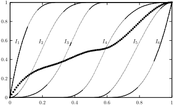
When one wants to enforce the monotonicity of function f, a standard approach is to use a basis of monotone spline functions, namely I-splines [Ramsay, 1988] denoted by Ii, i ∈ {1, . . . ,m}. For illustrative purpose, Fig. 1 shows a basis composed of six cubic I-spline functions, together with a spline function generated from this basis. As function u must be nondecreasing with u(0) = 0 and u(1) = 1, we define u as a convex combination of I-splines:
where λui ≥ 0 for all i ∈ {1, . . . ,m} and ∑mi=1 λui = 1. Similarly, since w is a nonincreasing function with w(0) = 1 and w(1) = 0, we define w by:
where λwi ≥ 0 for all i ∈ {1, . . . ,m} and ∑mi=1 λwi = 1. Equations 4 and 5 provide a compact definition of functions u and w using only 2m parameters, a number which remains constant as the number of lotteries increase. Without any knowledge of the DM's preferences, function u can be any function in U = {∑mi=1 λui Ii, (λu1 , . . . , λum) ∈ U}, where:
Similarly, w can initially be any element of the set W = {1- ∑mi=1 λwi Ii, (λw1 , . . . , λwm) ∈W}, where:
We now explain how this spline representation is used in our elicitation procedure. To this end, we show how values u(p), u(p), w(p) and w(p) are computed for any lottery p. By using our spline representation in Equation 2 (resp. 3), we observe that any uQuery (resp. wQuery) yields a linear constraint on parameters λui (resp. λwi ). Those linear constraints are then imposed to elements of U and W which are therefore characterized by linear constraints. Remark that sets U and W are two convex polyhedra that implicitly represent U and W at any time of the process.
Moreover, note that, for any lottery p, u(p) (resp. w(p)) is linear in parameters λui (resp. λwi ). Thus computing u(p) and w(p) can be achieved by solving the linear programs (LPs):
where LP Pu (resp. Pw) is used to minimize u(p) (resp. maximize w(p)). Note that Pw is here stated as a minimization problem because max{1-x} = 1-min{x}. Values u(p) and w(p) can similarly be obtained by changing the minimization problems into maximization problems.
5 Experiments
We carried out numerical tests in order to assess both the average number of queries required by our approach and the quality of the returned lottery. Interactions with the DM are simulated by generating answers to queries using WEU with two hidden, randomly generated, functions uh and wh. To model uh and wh, we use splines generated by a basis of m = 12 cubic I-spline functions as defined in Eq. 4, 5.
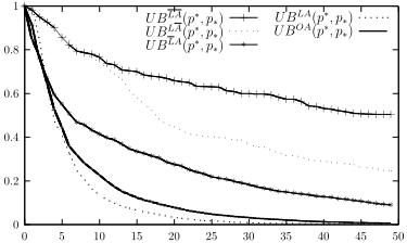
Number of queries. Our query generation strategy (described in the previous section and denoted by LA hereafter) is characterized by both the rule for selecting the lottery on which a query is asked and the rule for choosing the probability parameter α. In order to assess the impact of each of these rules, we investigate other strategies relaxing either the former and/or the latter. The different elicitation strategies obtained are denoted by LA, LA and LA, where L (resp. L) means that the queried lottery is chosen as in our strategy (resp. is chosen randomly) and A (resp. A) means that parameter α is chosen as in our strategy (resp. is chosen randomly). Finally, we also consider strategy OA that, instead of asking a query on the lotteries p∗ and p∗ , asks a query on the outcome (hence the O) in their support for which the value-imprecision is the highest; those queries are easier to answer for a DM as lotteries can be quite complex objects. We denote by UBS (p∗ , p∗) the upper bound obtained with strategy S, S ∈ {LA, LA,LA,LA}. Fig. 2a plots the decrease of UBS (p∗ , p∗) according to the number of queries averaged over 50 randomly generated sets L of possible lotteries. Each set L contains 1000 lotteries such that no stochastic dominance relation exist between them. The support of each lottery has a size generated uniformly in {1, . . . , 10} and consists of values generated uniformly in (0, 1). One observes that UBLA(p∗ , p∗) decreases efficiently; for instance, UBLA(p∗ , p∗) ≤ 0.05 after only 15 queries. If queries are issued on outcomes (strategy OA), the performance is slightly lower and 22 queries are required to reach
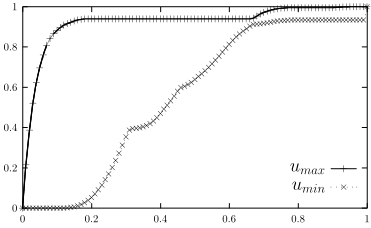
- (c) Minimal and maximal values that can be taken by the spline representing uh at the end of one run.
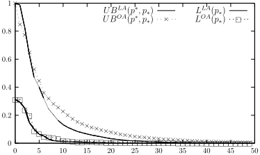
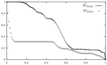
Figure 2: Results of the numerical tests for sets of 1000 lotteries.
UBOA(p∗ , p∗)=0.05. By contrast, the other strategies S are not able to reduce effectively UBS (p∗ , p∗).
Quality of the returned lottery. We recall that the bound UBS (p∗ , p∗) is a pessimistic estimate of the actual loss LS (p∗) that would be entailed by stopping the elicitation process and choosing lottery p∗:
Fig. 2b evaluates how far UBS (p∗ , p∗) is from LS (p∗) for S ∈ {LA,OA} (the two best strategies w.r.t. the number of queries). We observe that during the entire elicitation process, LS (p∗) is much lower than UBS (p∗ , p∗) for both S = LA and S = OA. In fact, LS (p∗) reaches 0 after only 10 queries for both elicitation strategies. This shows that, even if one decides an early interruption of the elicitation process (w.r.t. the estimate UBS (p∗ , p∗)), the chosen lottery p∗ is likely to be optimal w.r.t. uh and wh.
Interest of the incremental approach. In Fig. 2c and 2d, we plot the model that has been learned with our strategy on one run of 50 queries. The lines umin and umax (resp. wmin and wmax) give the minimal and maximal values that can be taken by the spline function u (resp. w) approximating uh (resp. wh) in each point according to the answers of the DM. Interestingly enough, it appears that functions u and w are far from being fully elicited, while the estimated loss is already tiny and lottery p∗ is almost surely optimal. This illustrates the main interest of the incremental approach that interweaves elicitation and optimization.
Computation time. We monitored the computation time required by our approach as it is crucial that the DM does not wait a prohibitively long time between two queries 5 . Even for a large set L consisting of 1400 lotteries, the overall computation time for 30 queries is 12sec. and, for instance, the 20th query requires less than 0.5sec (average times on 50 runs).
Other experiments. We tested how our approach is affected by varying the size of L and the maximum number of branches in the lotteries. Whichever strategy S is used, we did not observe a significant increase in the number of queries required to decrease efficiently UBS (p∗ , p∗).
6 Conclusion
We proposed an incremental elicitation procedure for the WEU model to solve the problem of identifying, within a given set of lotteries, a near-optimal solution. The efficiency of the method relies on a redefinition of functions u and w as monotone spline functions, which considerably reduces the elicitation burden while keeping a high descriptive power. Moreover, we have shown that, contrary to RDU, WEU has the strong advantage that functions u and w can easily be elicited concurrently in an incremental elicitation setting.
Acknowledgments
This work is supported by the ANR project CoCoRICoCoDec ANR-14-CE24-0007-01.
5 Implementation in Java using Gurobi 5.6.3 for the LPs. Times are wall-clock times on a 2.4 GHz Intel Core i5 with 8G of memory.
@inproceedings{ijcai2017p640,
  title     = {Incremental Decision Making Under Risk with the Weighted Expected Utility Model},
  author    = {Gilbert, Hugo and Benabbou, Nawal and Perny, Patrice and Spanjaard, Olivier and Viappiani, Paolo},
  booktitle = {Proceedings of the Twenty-Sixth International Joint Conference on
               Artificial Intelligence, {IJCAI-17}},
  publisher = {International Joint Conferences on Artificial Intelligence Organization},
  editor    = {Carles Sierra},
  pages     = {4588--4594},
  year      = {2017},
  month     = {8},
  note      = {Main track},
  doi       = {10.24963/ijcai.2017/640},
  url       = {https://doi.org/10.24963/ijcai.2017/640},
}
TY - CPAPER TI - Incremental Decision Making Under Risk with the Weighted Expected Utility Model AU - Gilbert, Hugo AU - Benabbou, Nawal AU - Perny, Patrice AU - Spanjaard, Olivier AU - Viappiani, Paolo T2 - Proceedings of the Twenty-Sixth International Joint Conference on Artificial Intelligence, IJCAI-17 PB - International Joint Conferences on Artificial Intelligence Organization PY - 2017 SP - 4588 EP - 4594 DO - 10.24963/ijcai.2017/640 UR - https://doi.org/10.24963/ijcai.2017/640 ER -Copied
Machine-readable versions of this paper, for tools and AI agents:





