
Fair and Efficient Social Choice in Dynamic Settings
Proceedings of the Twenty-Sixth International Joint Conference on Artificial Intelligence. Main track. Pages 4580-4587.
https://doi.org/10.24963/ijcai.2017/639
Keywords
- Uncertainty in AI: Sequential Decision Making
- Agent-based and Multi-agent Systems: Social Choice Theory
Abstract
We study a dynamic social choice problem in which an alternative is chosen at each round according to the reported valuations of a set of agents. In the interests of obtaining a solution that is both efficient and fair, we aim to maximize the long-term Nash social welfare, which is the product of all agents' utilities. We present and analyze two greedy algorithms for this problem, including the classic Proportional Fair (PF) algorithm. We analyze several versions of the algorithms and how they relate, and provide an axiomatization of PF. Finally, we evaluate the algorithms on data gathered from a computer systems application.
- [Agrawal and Devanur, 2015] Shipra Agrawal and Nikhil R Deva- nur. Fast algorithms for online stochastic convex programming. In Proceedings of the Twenty-Sixth Annual ACM-SIAM Sympo- sium on Discrete Algorithms, pages 1405-1424. SIAM, 2015.
- [Aleksandrov et al., 2015] Martin Aleksandrov, Haris Aziz, Serge Gaspers, and Toby Walsh. Online fair division: analysing a food bank problem. In Proceedings of the 24th International Joint Conference on Artificial Intelligence (IJCAI-15), 2015. IJCAI
- [Aziz et al., 2017] Haris Aziz, Markus Brill, Vincent Conitzer, Edith Elkind, Rupert Freeman, and Toby Walsh. Justified rep- resentation in approval-based committee voting. Social Choice and Welfare, 48(2):461-485, 2017.
- [Boutilier and Procaccia, 2012] Craig Boutilier and Ariel D Pro- caccia. A dynamic rationalization of distance rationalizability. In Proceedings of the Twenty-Sixth AAAI Conference on Artificial Intelligence, pages 1278-1284, 2012.
- [Brams et al., 2007] Steven J Brams, D Marc Kilgour, and M Remzi Sanver. A minimax procedure for electing committees. Public Choice, 132(3-4):401-420, 2007.
- [Caragiannis et al., 2012] Ioannis Caragiannis, Jason A. Covey, Michal Feldman, Christopher M. Homan, Christos Kaklamanis, Nikos Karanikolas, Ariel D. Procaccia, and Jeffrey S. Rosen- schein. On the approximability of Dodgson and Young elections. Artificial Intelligence, 187-188:31-51, 2012.
- [Caragiannis et al., 2014] Ioannis Caragiannis, Christos Kaklama- nis, Nikos Karanikolas, and Ariel D Procaccia. Socially desirable approximations for Dodgson's voting rule. ACM Transactions on Algorithms, 10(2): article 6, 2014.
- [Caragiannis et al., 2016] Ioannis Caragiannis, David Kurokawa, Hervé Moulin, Ariel D Procaccia, Nisarg Shah, and Junxing Wang. The unreasonable fairness of maximum Nash welfare. In Proceedings of the 17th ACM conference on Electronic Com- merce, pages 305-322, 2016.
- [Chamberlin and Courant, 1983] John R Chamberlin and Paul N Courant. Representative deliberations and representative deci- sions: Proportional representation and the Borda rule. American Political Science Review, 77(03):718-733, 1983.
- [Cole and Gkatzelis, 2015] Richard Cole and Vasilis Gkatzelis. Ap- proximating the Nash social welfare with indivisible items. In Proceedings of the Forty-Seventh Annual ACM on Symposium on Theory of Computing, pages 371-380. ACM, 2015.
- [Conitzer et al., 2017] Vincent Conitzer, Rupert Freeman, and Nis- arg Shah. Fair public decision making. In Proceedings of the 18th ACM Conference on Electronic Commerce, 2017. Forthcoming.
- [Darmann and Schauer, 2015] Andreas Darmann and Joachim Schauer. Maximizing Nash product social welfare in allocating indivisible goods. European Journal of Operational Research, 247(2):548-559, 2015.
- [Elkind et al., 2014] Edith Elkind, Piotr Faliszewski, Piotr Skowron, and Arkadii Slinko. Properties of multiwinner voting rules. In Proceedings of the Thirteenth International Conference on Autonomous Agents and Multiagent Systems, pages 53-60, 2014.
- [Ghodsi et al., 2011] Ali Ghodsi, Matei Zaharia, Benjamin Hind- man, Andy Konwinski, Scott Shenker, and Ion Stoica. Dominant resource fairness: Fair allocation of multiple resource types. Pro- ceedings of the 8th USENIX conference on Networked systems design and implementation, pages 24-24, 2011.
- [Guo et al., 2009] Mingyu Guo, Vincent Conitzer, and Daniel M. Reeves. Competitive repeated allocation without payments. In Proceedings of the Fifth Workshop on Internet and Network Eco- nomics (WINE), pages 244-255, Rome, Italy, 2009.
- [Jalali et al., 2000] A. Jalali, R. Padovani, and R. Pankaj. Data throughput of CDMA-HDR a high efficiency-high data rate personal communication wireless system. In Proceedings of the IEEE Vehicular Technology Conference, pages 1854-1858. IEEE, 2000.
- [Kash et al., 2014] Ian Kash, Ariel D Procaccia, and Nisarg Shah. No agent left behind: Dynamic fair division of multiple re- sources. Journal of Artificial Intelligence Research, pages 579- 603, 2014.
- [Monroe, 1995] Burt L Monroe. Fully proportional representation. American Political Science Review, 89(04):925-940, 1995.
- [Nash, 1950] John Nash. The bargaining problem. Econometrica, 18(2):155-162, 1950.
- [Nemhauser and Wolsey, 1988] George L Nemhauser and Lau- rence A Wolsey. Integer and combinatorial optimization. inter- science series in discrete mathematics and optimization. ed: John Wiley & Sons, 1988.
- [Parkes and Procaccia, 2013] David C Parkes and Ariel D Procac- cia. Dynamic social choice with evolving preferences. In Pro- ceedings of the Twenty-Seventh AAAI Conference on Artificial In- telligence, pages 767-773, 2013.
- [Parkes et al., 2010] David C Parkes, Ruggiero Cavallo, Florin Constantin, and Satinder Singh. Dynamic incentive mechanisms. AI Magazine, 31(4):79-94, 2010.
- [Parkes et al., 2012] David C Parkes, Ariel D Procaccia, and Nis- arg Shah. Beyond dominant resource fairness: Extensions, lim- itations, and indivisibilities. In ACM Conference on Electronic Commerce, pages 808-825. ACM, 2012.
- [Procaccia, 2013] Ariel D Procaccia. Cake cutting: not just child's play. Communications of the ACM, 56(7):78-87, 2013.
- [Ramezani and Endriss, 2010] Sara Ramezani and Ulle Endriss. Nash social welfare in multiagent resource allocation. In Agent- Mediated Electronic Commerce. Designing Trading Strate- gies and Mechanisms for Electronic Markets, pages 117-131. Springer, 2010.
- [Viswanath et al., 2002] Pramod Viswanath, David NC Tse, and Rajiv Laroia. Opportunistic beamforming using dumb anten- nas. IEEE Transactions on Information Theory, 48(6):1277- 1294, 2002.
- [Zaharia et al., 2010] Matei Zaharia, Mosharaf Chowdhury, Michael J Franklin, Scott Shenker, and Ion Stoica. Spark: Cluster computing with working sets. In Proceedings of the 2nd USENIX Conference on Hot Topics in Cloud Computing, volume 10, page 10, 2010.
References were extracted automatically from the PDF and may contain errors.
Full text extracted automatically from the PDF; figures, tables and equations may differ. The PDF is the version of record.
1 Introduction
Fairness is a topic of rapidly increasing interest in social choice. On the one hand, there has been much recent interest in the fair allocation of resources-cake cutting [Procaccia, 2013] as well as other models [Ghodsi et al., 2011; Parkes et al., 2012]. On the other hand, in voting, fairness considerations have received attention in selecting a committee, in the form of a focus on the voters being represented in the committee [Chamberlin and Courant, 1983; Monroe, 1995; Brams et al., 2007; Aziz et al., 2017].
A classical approach to obtaining a fair outcome in a context where agents have utility functions is to maximize the Nash welfare [Nash, 1950], which is the product of the agents' utilities. One attractive feature of using the maximum Nash welfare (MNW) solution is scale invariance: if an agent doubles all her utilities (or, equivalently, changes the units in which she expresses her utilities), this does not change which outcomes maximize the objective (the solution is not however stable under additive transformations, where an agent simply adds some constant value to all her reported utilities).
In life, it is often difficult to make a completely fair decision in a single-shot context; often, every option will leave some agents unhappy. Fortunately, we can often address this over time-we will go to my most preferred restaurant today, and to yours next week. Achieving fairness over time is the topic of our paper. Ours is certainly not the first work to consider fairness or social choice in dynamic settings [Parkes and Procaccia, 2013; Kash et al., 2014; Aleksandrov et al., 2015].
When we make multiple decisions over time, we could simply maximize the Nash welfare in each round separately. But it is easy to see that this can lead to dominated outcomes. For example, suppose there are two agents, and we can choose an alternative that gives one a reward of 3, and the other a reward of 0; or vice versa; or an alternative that gives each of them 1. Within a round, the last alternative maximizes Nash welfare; but if this scenario is repeated every round, then it would be better to alternate between the first two alternatives, so that each agent obtains 1.5 per round on average. Of course, initially, say in the first round, we may not realize we will have these options every round, and so we may choose the last alternative; but if we do have these options every round, we should eventually catch on to this pattern and start alternating. Ideally, we would maximize the long-term Nash welfare, that is, the product of the long-run utilities (which are the sums of each agent's rewards), rather than, for example, the sum of the products within the rounds.
In this work, we do not focus primarily on strategic concerns. Of course it is fairly common to ignore strategic concerns in the social choice literature, but we do think this is an important topic for future work. On the other hand, there are also important contexts where strategic concerns do not come into play. For example, instead of considering a setting where there are multiple agents that have different utility functions, we can consider a setting where there are multiple objectives that each alternative contributes towards. For example, consider faculty hiring. Suppose the three objectives that we want our faculty hires to contribute to are research, teaching, and service; moreover, suppose that at the time of hiring we can predict well how much each candidate would contribute to each of these objectives, if hired. Then, it stands to reason that, one year, we may hire a top researcher that we do not expect to contribute much to the other objectives. But we would be loath to make such a decision every year; having hired a few top researchers who are not good at teaching or service, pressure will mount to address these needs. This fits well into our framework, if we simply treat each of the three objectives as an agent that is "happy" with an alternative to the extent to which it addresses the corresponding objective.
The rest of the paper is organized as follows. In Section 2 we introduce notation and preliminaries. In Section 3 we present two simple greedy algorithms for choosing alternatives, and provide intuitive interpretations of them, including an axiomatic justification for one of them. After presenting the algorithms, we evaluate them on data from a computer systems application in Section 4.
Justification for Nash welfare: The Nash welfare is frequently used as an objective in the fair division literature as it strikes a balance between maximizing efficiency and fairness [Cole and Gkatzelis, 2015; Darmann and Schauer, 2015; Ramezani and Endriss, 2010]. Caragiannis et al. [2016] have recently shown the MNW solution to satisfy envy freeness up to one good, as well as approximating the maximin share guarantee. However, work in fair division focuses primarily on the allocation of private goods, where each alternative gives utility to exactly one agent. This is not the case in our setting, where each alternative can be valued positively by many agents. Conitzer et al. [2017] explicitly consider fairness axioms in the public good setting, including proportionality, which states that each agent should derive at least a 1n fraction of the utility she could obtain by choosing the outcome at each round. It turns out that a proportional solution may not exist in our setting, but the MNW solution always satisfies a weaker criterion: For each agent i, there exists a round such that if i is given control of that round, then i achieves their utility guaranteed by proportionality.
We can also appeal to Nash's original axiomatization of the MNW solution [Nash, 1950] as the only solution that satisfies scale-freeness, Pareto optimality, independence of irrelevant alternatives, and symmetry, which are all natural in our setting (although without an explicit focus on fairness).
Related work: Parkes and Procaccia [2013] examine a similar problem by modeling agents' evolving preferences with Markov Decision Processes, with a reward function defined over states and actions (alternatives). However, their goal is to maximize the sum of (discounted) rewards and they do not explicitly consider fairness as an objective. Kash et al. [2014] examine a model of dynamic fair division where agents arrive at different times and must be allocated resources; however, they do not allow for the preferences of agents to change over time as we do. Aleksandrov et al. [2015] consider an online fair division problem in a setting where items appear one at a time, and agents declare yes/no preferences over that item. In our setting, each round has many alternatives and agents express more general utilities. Our work is related to the literature on dynamic mechanism design (Parkes et al. [2010] provide an overview), except that we do not consider monetary transfers. Guo et al. [2009] consider a setting similar to ours, also without money, except that they are not explicitly interested in fairness, only welfare, and focus on incentive compatibility.
2 Preliminaries
Consider a set of n agents and let A = {a1, . . . , am} be a set of m possible alternatives. 1 At every round t = 1, . . . , T, every agent i reports her valuation vt i (aj) ∈ N for every alternative aj. 2 Thus the input at every round is a matrix V t = (vt i (aj))ij. Let vt (aj) denote the j-th column of matrix V t , the vector of valuations for alternative aj. For every round t, a Dynamic Social Choice Function (DSCF) chooses a set of alternatives Ct, from which a single alternative ct is chosen arbitrarily. Importantly, the problem is online, so we may only use information up to time t in order to choose Ct.
1 For simplicity of presentation, we define the set of alternatives to be static. However, all of our algorithms and results hold if the set, and even the number, of alternatives changes from round to round.
We define a vector of accrued rewards at round t, ut, where the accrued reward of agent i at round t is the sum of i's valuations for the chosen alternatives up to and including round t, ut(i) = ∑tt′=1 vt′ i (ct′). We will often be interested in an agent's accrued reward before the start of round t, ut-1(i). For convenience, we will refer to the set of agents with ut-1(i) = 0 by I0 when the round, t, is clear. The average utility of the agents over the first t rounds is uavg t = 1t ut.
A DSCF is anonymous if applying permutation σ to the agents, for all t, does not change the set of chosen alternatives Ct, for any t. A DSCF is neutral if applying permutation σ to the alternatives, for all t, results in choosing alternatives σ(Ct) for all t. For the rest of this paper we only consider anonymous, neutral DSCFs.
The Nash welfare (NW) of valuation vector u, NW(u), is defined to be the product of the agents' utilities, NW(u) = ∏ni=1 u(i). We also define NW +(u) = ∏i:u(i)̸=0 u(i) to be the product of all positive entries of u. Our aim is to maximize the NW of the average utility across all T rounds, NW(uavg T ). Note that while our setting allows for discounting, we do not need to explicitly address it since the input matrices can be pre-multiplied by the necessary factor before being passed as input to the DSCF.
The benchmark algorithm is the optimal algorithm for the offline problem, where an instance is given by the set {V t }t∈{1,...,T}, and can be solved by a mixed integer convex program. We denote the optimal Nash welfare by OPT.
Our algorithms and analysis use a formal infinitesimal quantity ϵ. Numbers involving ϵ take the form ∑i=∞ i=-∞ aiϵi . 3 For two such numbers a = ∑i=∞ i=-∞ aiϵi and b = ∑i=∞ i=-∞ biϵi , let i′ be the smallest index for which ai ̸= bi, if it exists. Then a > b if and only if ai′ > bi′ . That is, we compare numbers lexicographically by the lowest powers of ϵ. Two numbers are equal if all coefficients are equal.
Many proofs, as well as additional simulations, are omitted due to space constraints. The details can be found in the full version of the paper, which appears on the authors' websites.
3 Greedy Algorithms
3.1 AlgorithmDefinitions
In this section we present two greedy algorithms. We note that, although these algorithms are designed to give an approximate solution to that which maximizes Nash welfare, much of this section is devoted to showing that they satisfy desirable properties as algorithms in their own right. Such an approach is not new in computational social choice - for other papers that treat approximation algorithms as distinct voting rules see, for example, [Caragiannis et al., 2012; 2014; Elkind et al., 2014]. The first algorithm, GREEDY, simply chooses ct to maximize NW(uavg t ), the Nash welfare at the end of the round. The second algorithm is a linearized version of greedy known as PROPORTIONALFAIR (PF) in the networking community [Viswanath et al., 2002; Jalali et al., 2000], which maximizes the sum of percentage increases in accrued reward at each round. Equivalently, it works by assigning each agent a weight wi (denote the vector of weights by w) equal to the inverse of her accrued reward at the start of each round and chooses Ct = argmaxaj∈A w·vt (aj), the alternatives that maximize the weighted sum of valuations. Note that wi is proportional to the product of the other agents' accrued rewards.
2 Restricting valuations to be non-negative integers is necessary for some of our results in Section 3. This is still sufficient for agents to express their preferences to arbitrary levels of precision.
3 While our framework allows for unbounded powers of ϵ, in this paper we utilize only powers of ϵ between ϵ-1 and ϵn .
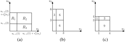
Example 1. Let n = m = 2 and suppose that ut-1(1) = 1, ut-1(2) = 3, and V t = ( 2 3 3 1 ). That is, agent 1 has valuation 2 for alternative a1 and valuation 3 for alternative a2. Agent 2 has valuation 3 for alternative a1 and valuation 1 for alternative a2. Choosing a1 results in Nash welfare of (1 + 2) · (3 + 3) = 18, while choosing a2 results in Nash welfare of (1+3) · (3+1) = 16. Thus GREEDY chooses a1.
Under PF, each agent is given weight inversely proportional to their own accrued utility. That is, agent 1 has weight 1 and agent 2 has weight 1 3 . Now, taking the weighted sum of valuations yields (1 · 2) + ( 13 · 3) = 3 for alternative a1, and (1 · 3) + ( 1 3 · 1) = 10 3 for alternative a2. Thus PF chooses a2.
A graphical illustration of the difference between the two algorithms is given in Figure 1.
Unfortunately, both algorithms encounter problems while there exist agents with zero accrued reward. For GREEDY, it can (and, unless some alternative is valued positively by all agents, will) be the case that NW(uavg t ) = 0 for all choices of ct, even when one alternative is weakly preferred to all other alternatives by all agents. For PF, it is impossible to set a weight wi = 1 ut-1(i) for an agent with ut-1(i) = 0.
As a general framework for addressing this issue, we endow each agent i ∈ I0 with some arbitrary, infinitesimal reward at the start of each round. This is a natural way to allow the algorithms to give high priority to agents with zero accrued reward while avoiding mathematical inconsistencies, and it allows us to efficiently choose an alternative ct if we are happy with selecting any member of the choice set Ct.
However, once we endow rewards (even infinitesimal ones), we immediately lose scale-freeness, one of the appealing properties of using Nash welfare. Further, if we want to choose a member of the choice set Ct uniformly at random, there is no obvious distribution over endowed rewards that allows us to do this - choosing endowed rewards uniformly at random from some interval will not, in general, result in drawing uniformly from Ct. So, while the technique of randomly endowing infinitesimal reward is a general and intuitive way for the algorithms to handle all situations, we also want an algorithm to compute the entire choice set Ct.
In the following, for both GREEDY and PF, we first present the algorithm to select a single alternative via nondeterministically endowing infinitesimal reward, followed by an algorithm to compute the entire choice set Ct.
Algorithm 1 GREEDY (select one alternative)
- 1: Input ut-1 2: for i = 1, . . . , n do 3: Randomly choose 0 < xi ≤ 1 4: end for 5: Return ct ∈ argmaxaj∈A ∏ni=1 max{ut-1(i) + vt i (aj ), xiϵ}
The alternatives chosen by Algorithm 1 are exactly the alternatives that result in a maximal number of agents with positive accrued reward and, subject to holding fixed the set of agents with positive accrued reward, maximizes the product of these agents' rewards.
Algorithm 2 GREEDY (select all alternatives)
- 1: Input ut-1 2: Ct ← argmaxaj∈A |{i : ut-1(i) + vt i (aj ) > 0}| 3: for j ∈ Ct do 4: if ∃j ′ such that 5: {i : ut-1(i)+vt i (aj) > 0} = {i : ut-1(i)+vt i (aj ′ ) > 0} and NW +(ut-1+vt (aj)) < NW +(ut-1+vt (aj ′ )) then 6: Ct ← Ct\{aj} 7: end if 8: end for 9: Return Ct
The version of PF for selecting a single alternative is presented as Algorithm 3.
To determine the complete choice set Ct, we solve a linear program for each alternative that explicitly determines whether there is some infinitesimal endowment that results in the alternative being chosen by PF.
A notable difference in the algorithms is that unlike GREEDY, PF may leave some agents with zero accrued utility
Algorithm 3 PROPORTIONALFAIR (select one alternative)
- 1: Input ut-1
- 2: for i ∈ I0 do
- 3: Randomly choose 0 < xi ≤ 1
- 4: Randomly choose yi ∈ R
- 5: end for
- 7: Return ct ∈ argmaxaj∈Aw · vt (aj)
Algorithm 4 PROPORTIONALFAIR (select all alternatives)
- 1: Input ut-1
- 2: Ct ← ∅
- 3: for j = 1, . . . ,m do
- 4: if the following linear program is unbounded
Maximize L
then
- 6: end if
- 7: end for
- 8: Return Ct
even when it was possible to give positive utility to all agents.
Example 2. Let n = 2, m = 3, and t = 1. Suppose that V1 = ( 3 0 1 0 3 1 ). Because t = 1, ut-1(1) = ut-1(2) = 0.
GREEDY chooses a3 since it is the only alternative that provides non-zero reward to both agents. However, PF assigns the agents weights w1,w2 and chooses argmaxj∈{1,2,3}w · vt (aj). Since it must be the case that either 3w1 > w1 + w2 or that 3w2 > w1 + w2, it is not possible for a3 to be chosen by PF.
For each algorithm, we prove equivalence of the two versions in the sense that the set generated by the 'select all' version consists exactly of the alternatives that the 'select one' version generates for some nondetermistic choices.
Theorem 1. The set of alternatives Ct chosen by Algorithm 2 at round t is exactly the set of alternatives that can be chosen at round t by Algorithm 1.
The proof uses the fact that the product on Line 5 of Algorithm 1 is maximized when the number of ϵ terms appearing in the product is minimized.
Theorem 2. The set of alternatives Ct chosen by Algorithm 4 at round t is exactly the set of alternatives that can be chosen at round t by Algorithm 3.
Proof. We begin by showing that every alternative that can be selected by Algorithm 3 is also selected by Algorithm 4. Let ct be an alternative chosen by Algorithm 3 for some choices of {xi}i∈I0 and {yi}i∈I0 . For all i ̸∈ I0, set w′i = 1 ut-1(i) , and for all i ∈ I0, set w′i = xi δ + yi for any δ > 0. As δ → 0, the variables w′i grow arbitrarily large. Therefore, to show feasibility of the variables {w′i } we need to show that the first set of constraints in the LP in Algorithm 4 hold for sufficiently small δ.
Fix an alternative aj. From Line 7 of Algorithm 3, we know that w·vt (ct) ≥ w·vt (aj). The dominant coefficient in this expression is that of ϵ-1 . Comparing these coefficients gives us
If Inequality 1 is strict, then we know that ∑i∈I0 xi δ vt i (ct) > ∑i∈I0 xi δ vt i (aj) for any δ > 0, and we can make the gap arbitrarily large by setting δ sufficiently small. In particular, we can force the gap to be large enough that the following inequality holds for any fixed values of {yi}i∈I0 and {ut-1(i)}i̸∈I0 :
which is precisely the first constraint in the linear program from Algorithm 4.
If Inequality 1 holds with equality, then we turn attention to the coefficient of ϵ0 in the dot product from Line 7 of Algorithm 3. This tells us that
Dividing Inequality 1 by δ and adding Inequality 2 gives ∑ni=1 w′i vt i (ct) ≥ ∑ni=1 w′i vt i (aj), satisfying the first constraint of the LP, so the weights {w′i } are feasible. These weights allow us to set L to arbitrarily large values as δ → 0, so the LP is unbounded and Algorithm 4 selects ct.
We now show the other direction, that every alternative selected by Algorithm 4 can also be selected by Algorithm 3. Let ct ∈ Ct. That is, the optimal value for the LP in Algorithm 4 is unbounded. Then it is the case that there exist vectors p and q ̸= 0 for the values of the variables in the LP such that p + kq is feasible for all k > 0 and q has positive objective value (this is a known fact about linear programs with unbounded value; see, e.g., [Nemhauser and Wolsey, 1988], Theorem 4.7). We use these to exhibit values of {xi}i∈I0 and {yi}i∈I0 so that ct is chosen by Algorithm 3.
Set yi = pi and xi = qi for all i ∈ I0. Let aj ∈ A. By the first set of constraints from the LP,
for all k > 0. In particular, this implies that it can not be the case that ∑i∈I0 qivt i (ct) < ∑i∈I0 qivt i (aj), or else Inequality 3 would be violated for large enough values of k. There are two possiblities.
First, suppose that ∑i∈I0 qivt i (ct) > ∑i∈I0 qivt i (aj ). Then, by our choice of xi = qi for all i ∈ I0, we have that ∑i∈I0 xivt i (ct) > ∑i∈I0 xivt i (aj). But, as discussed earlier, ∑i∈I0 xivt i (aj) is exactly the dominant term in Line 7 of Algorithm 3. Therefore, this dot product is maximized by ct, so ct is chosen by Algorithm 3.
Finally, suppose that ∑i∈I0 qivt i (ct) = ∑i∈I0 qivt i (aj ). So the dominant term in Line 7 of Algorithm 3 is equal for ct and aj. By Inequality 3, it must be the case that
By the choice of yi = pi for all i ∈ I0, the above inequality holds when we substitute yi for every instance of pi. After making that substitution, we are left with exactly the expression for the coefficient of ϵ0 in Line 7 of Algorithm 3. Since the coefficient is at least as large for ct as for aj, and the ϵ-1 coefficients are equal (and there are no further non-zero terms), ct may be chosen by Algorithm 3.
3.2 Axiomatization of PROPORTIONALFAIR
Now that we have given a precise definition of the PF mechanism and justified it, in this section we provide an axiomatization of the PF mechanism.
A DSCF is scale-free if it is not affected by a uniform (multiplicative) scaling of some agent's valuations. This property is desirable because it means we do not require any sort of agreement or synchronization as to the units of measurement used by the agents in their reporting.
Definition 1. Let k > 0. Say that a DSCF satisfies scale-freeness (SF) if Ct is unchanged (for the same choice of tiebreaking in earlier rounds) if we replace vt i (aj ) by k · vt i (aj) for all aj ∈ A for every t = 1, . . . , T .
A DSCF is separable into single-minded agents if the chosen alternative at a round is unchanged by replacing an agent by several new agents with the same accrued reward, each of which has unit positive valuation for only one alternative. The axiom reflects that we can interpret utilities cardinally rather than just ordinally.
Definition 2. Say that a DSCF is separable into singleminded agents (SSMA) if, when all agents have the same accrued utility ut-1(i) = u > 0, Ct is unchanged if we replace each agent with several new agents (denoted generically by x) according to the following scheme: For every vt i (aj) ∈ V t , create vt i (aj) agents each with ut-1(x) = u, vtx (aj) = 1, and vtx (aj ′ ) = 0 for all j ′ ̸= j.
The plurality axiom says that if all agent valuation vectors are unit vectors, and we have no reason to distinguish between agents, then the alternatives favored by the most agents should be chosen.
Definition 3. Say that a DSCF satisfies plurality (P) if, when all agents have unit valuation for only a single alternative, and all agents have the same (non-zero) accrued utility, then Ct consists of the alternatives with non-zero valuation from the most agents.
Plurality says nothing about the case when some agent has ut-1(i) = 0. The idea of the axiom (in combination with SF) is that we should choose the alternative which provides the greatest utility, relative to what agents already have. However, if agents have zero accrued reward then it is not possible to make accurate comparisons as to the relative benefit each agent receives.
The final axiom says that, if we restrict attention to only agents with zero accrued reward, alternatives which are dominated by a mixture of other alternatives should not be played. In the case that two alternatives are equivalent with respect to agents with ut-1(i) = 0, we should only choose an alternative if it would still be chosen in the absence of the agents with ut-1(i) = 0. The definition is inspired by mixed strategy dominance in game theory and, intuitively, formalizes that we should prioritize agents with zero utility above all others.
We first define the notion of 0-dominance.
Definition 4. Let z1, . . . , zm be nonnegative coefficients with ∑j ′ zj ′ = 1. We say that an alternative aj is strictly 0dominated by the mixture of alternatives ∑j ′ zj ′aj ′ at round t if ∑j ′ zj ′vt i (aj ′ ) ≥ vt i (aj ) for all agents i with ut-1(i) = 0, with at least one of these inequalities being strict. If all inequalities hold with equality, then we say that aj is weakly 0-dominated by the mixture ∑j ′ zj ′aj ′ .
We say that aj is (strictly, weakly) 0-dominated if there exists some mixture of alternatives that (strictly, weakly) 0dominates it.
Definition 5. A DSCF f satisfies No 0-Dominated Alternatives (NZDA) if it never chooses a strictly 0-dominated alternative, and chooses a weakly 0-dominated alternative aj only if aj would be chosen by f under a scenario where V t was modified to include (1) only the agents with ut-1(i) > 0, and (2) only the (mixtures of) alternatives that weakly 0-dominate aj (including aj itself).
Lemma 1. PF satisfies SF, SSMA, P, and NZDA.
We now show that any mechanism that achieves SF, SSMA, P, and NZDA simultaneously must agree with PF. We note that of the four axioms, GREEDY satisfies only SF and P. Despite GREEDY being (arguably) simpler than PF, we do not know a good axiomatization for it.
Theorem 3. Let f be a DSCF that satisfies SF, SSMA, P, and NZDA. Suppose that f chooses alternative ct at round t. Then PF must also choose ct at round t (for the same history up to that point).
Proof. We have already shown that PF satisfies SF, SSMA, P, and NZDA. It remains to show that f's choice of alternative can also be chosen by PF. In the case that all agents have ut-1(i) > 0, we use the fact that f satisfies SF, SSMA, and P to show that f's choice of alternative is the same as one chosen by PF. First we use SF to scale the agents' accrued utilities to be the same (since they are all non-zero), then use SSMA to replace each agent with several new agents which have unit vector valuations, and then use plurality to choose ct (which can be shown to coincide with that chosen by PF). Due to space constraints, we omit the details.
The more intricate case is when there exists at least one agent with ut-1(i) = 0. Since f satisfies NZDA, we know that f never chooses a strictly 0-dominated alternative and only chooses a weakly 0-dominated alternative if f would still choose that alternative when V t is modified according to Definition 5. To complete the proof, we show that PF selects all alternatives that can possibly be chosen by f. Specifically, we show that PF can choose all alternatives that are not (strictly or weakly) 0-dominated, as well as any weakly 0-dominated alternative aj ∗ that is chosen by PF for the modified V t . That is, when all alternatives are removed other than aj ∗ and (mixtures of) alternatives that weakly 0-dominate it, and all agents with ut-1(i) = 0 are removed. This is sufficient since we have shown that PF chooses every alternative chosen by f when all agents have ut-1(i) > 0 (which is the case when all agents with ut-1(i) = 0 are removed).
An alternative aj ∗ is either (a) strictly 0-dominated, or (b) weakly 0-dominated and not chosen by PF when V t is modified according to Definition 5, if and only if the optimal value of the following LP is negative for arbitrarily large values of H. We omit the index of the round t from the agents' valuations for clarity.
If aj ∗ is strictly dominated then the first term of the objective can be made negative (and therefore the whole objective can be made negative when H is large enough). If aj ∗ is only weakly dominated, then the first term can be set to 0, and the second term to be negative when there exists a mixture of alternatives that is chosen by PF (ahead of aj ∗) according to the modified V t . Conversely, if the optimal value of the objective is negative then either there exist values for {zj} such that the first term is negative (which, combined with the first set of constraints, says that aj ∗ is strictly 0-dominated), or there exist values for {zj} such that the first term is zero and the second term is negative. If the second term is negative then the weighted sum of valuations for the mixed alternative defined by {zj} is higher than the weighted sum of valuations for aj ∗, for the weights defined by PF when restricted to agents i ̸∈ I0. This proves correctness of the LP.
We want to show that PF can choose any alternative for which the the optimal value of LP (4) is nonnegative. Let aj ∗ be such an alternative. We show that aj ∗ can be chosen by PF by considering the dual, which has variables wi for all i ∈ I0 (one for each constraint) and r (corresponding to the constraint on the sum of the zj):
| Category | Applications |
|---|---|
| Statistics | Correlation |
| Classification | DecisionTree, GradientBoostedTrees, SVM, LinearRegression, NaiveBayesian |
| Pattern Mining | FP Growth |
| Clustering | KMeans |
| Collaborative Filtering | ALS |
| Graph Processing | Pagerank, ConnectedComponents, TriangleCounting |
Let r = ∑i∈I0 vi(aj ∗)wi - r denote the objective. The first set of constraints can now be rewritten as
Since aj ∗ is not 0-dominated, the optimal value of LP (4) is at least zero for any arbitrarily large value of H. By strong duality, the optimal value of the dual is therefore also at least zero for arbitrarily large values of H. Thus, if we set w′i = wi + H for all i ∈ I0 and w′i = 1 ut-1(i) for all i ∈ I0, we have an unbounded and feasible set of weights for the linear program to choose aj ∗ in the definition of Algorithm 4. Therefore, aj ∗ can be chosen by PF.
4 Simulations
We ran the algorithms on data gathered from a power boost allocation problem. In this problem, n computer applications are each allocated a base level of power, and compete for m < n additional (indivisible) units of extra power (power boosts) at each of T rounds (each application gets at most one boost per round). We obtain our instance from Apache Spark [Zaharia et al., 2010] benchmarks.
Table 1 lists the twelve Spark applications in our instance, each of which is defined by a fixed number of tasks. We profile tasks' completion time. We take the number of tasks completed in a round by an application as that application's utility. Thus, for each application a, we estimate the base and boosted power utility (ubase a,t and uboost a,t ) in each round.
In our instance, there are two power boosts to be allocated. So at each round there are (12 2 ) alternatives, one for each pair of applications. For an alternative j corresponding to power boosts for applications a and b, we have that vta (j) = uboost a,t , vtb (j) = uboost b,t , and vtc (j) = ubase c,t for all other applications c ̸= a, b. We have 497 rounds in the instance we tested.
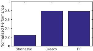
We evaluate the performance of GREEDY and PF against the optimal offline solution, and also against an algorithm designed for online stochastic convex programming 4 [Agrawal and Devanur, 2015] - a class of problems that includes the one we study. To our knowledge this algorithm is the state of the art for such problems in terms of theoretical guarantees. We refer to this algorithm as STOCHASTIC. The algorithm works by maximizing a weighted sum of valuations at each round, where the weights are updated at each round using online convex optimization techniques. The theoretical guarantees for STOCHASTIC are in expectation over instances where the order of the input matrices is randomly permuted. In the instance we test, however, the utilities are highly correlated over time. Applications that would benefit from a power boost in some round t are more likely to also benefit from a power boost in round t + 1, because application phases may span multiple rounds. Due to this and other technical reasons, the theoretical guarantees do not apply here. The performance of the three algorithms is shown in Figure 2.
We see that STOCHASTIC performs relatively poorly, while GREEDY and PF each achieve about 80% of the performance of OPT. This motivates us to examine the difference in performance between GREEDY and PF for smaller values of T , as the difference between these two algorithms is most pronounced while a single decision has a relatively large effect.
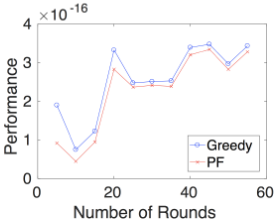
To generate smaller instances, we sample starting rounds from the full set of 497 rounds. For each value of T in Figure 3, we randomly generate a starting round t ∈ [1, 497-T ] and consider the T rounds starting at t, for 100 random choices of t. Our measure of performance is NW(uavg T ), allowing for fair comparisons between different values of T .
We note that PF consistently performs slightly worse than GREEDY, which is consistent with the performance on the full instance. The difference is most pronounced on small values of T, since this is where the two algorithms differ the most. Performance increases with T, as we would expect, since more rounds allow the algorithms to choose more flexibly once all applications have positive accrued reward. However, the increase is not monotonic. One explanation for this is because we throw away any choice of starting round t for which it is impossible to achieve NW(uavg T ) > 0 (it might be the case that for all T rounds, some application cannot receive positive utility). Since smaller values of T result in more choices of t being disqualified, there is a sense in which we are selecting for 'easier' instances for smaller values of T .
4 Of course, there are other online scheduling algorithms but they do not pursue Nash welfare as an objective.
5 Conclusion
Election designers and social choice researchers often do not consider the fact that many elections do not occur in isolation, but rather are repeated over time. In this work, we have provided a framework to allow for the design and analysis of dynamic election protocols, and repeated decision making rules generally. We have presented two candidate online algorithms for solving these dynamic problems. Our simulations show that both algorithms perform well, but do not determine that either is clearly a better choice than the other. While GREEDY achieves slightly higher performance, PROPORTIONALFAIR has the advantage of being justified by the axiomatization given in this paper.
Our work leaves a lot of scope for future research. One direction would be to design a more precise model of voter preferences, possibly modeling changing preferences by an MDP [Boutilier and Procaccia, 2012; Parkes and Procaccia, 2013]. We have also not considered modeling discounting of the agents' utilities. Finally, there are many interesting questions regarding strategic behavior by the agents. In the most general setting, there appears to be no hope for a fair, strategy-proof rule due to the free-rider problem: agents are incentivized to under-report their utility for an alternative that gets chosen, and are thus indistinguishable from an agent that is genuinely unhappy with the chosen alternative. However, it may be possible to regain some (limited) strategy-proofness in a more restricted setting. For instance, what if we place restrictions on the utilities that can be reported, or restrict our attention to private goods?
Acknowledgments
We sincerely thank Songchun Fan for sharing the data used in Section 4, and Andrew Kephart for helpful discussions. We are thankful for support from NSF under awards IIS1527434, IIS-0953756, CCF-1101659, CCF-1149252 (CAREER), CCF-1337215 (XPS-CLCCA), SHF-1527610, and AF-1408784, ARO under grants W911NF-12-1-0550 and W911NF-11-1-0332, and a Guggenheim Fellowship. This work is also supported by STARnet, a Semiconductor Research Corporation program, sponsored by MARCO and DARPA. This work was done in part while Conitzer was visiting the Simons Institute for the Theory of Computing. Any opinions, findings, conclusions, or recommendations expressed in this material are those of the authors and do not necessarily reflect the views of these sponsors.
@inproceedings{ijcai2017p639,
  title     = {Fair and Efficient Social Choice in Dynamic Settings},
  author    = {Freeman, Rupert and Zahedi, Seyed Majid and Conitzer, Vincent},
  booktitle = {Proceedings of the Twenty-Sixth International Joint Conference on
               Artificial Intelligence, {IJCAI-17}},
  publisher = {International Joint Conferences on Artificial Intelligence Organization},
  editor    = {Carles Sierra},
  pages     = {4580--4587},
  year      = {2017},
  month     = {8},
  note      = {Main track},
  doi       = {10.24963/ijcai.2017/639},
  url       = {https://doi.org/10.24963/ijcai.2017/639},
}
TY - CPAPER TI - Fair and Efficient Social Choice in Dynamic Settings AU - Freeman, Rupert AU - Zahedi, Seyed Majid AU - Conitzer, Vincent T2 - Proceedings of the Twenty-Sixth International Joint Conference on Artificial Intelligence, IJCAI-17 PB - International Joint Conferences on Artificial Intelligence Organization PY - 2017 SP - 4580 EP - 4587 DO - 10.24963/ijcai.2017/639 UR - https://doi.org/10.24963/ijcai.2017/639 ER -Copied
Machine-readable versions of this paper, for tools and AI agents:





