
Adaptive Hypergraph Learning for Unsupervised Feature Selection
Proceedings of the Twenty-Sixth International Joint Conference on Artificial Intelligence. Main track. Pages 3581-3587.
https://doi.org/10.24963/ijcai.2017/501
Keywords
- Machine Learning: Feature Selection/Construction
- Machine Learning: Machine Learning
- Machine Learning: Unsupervised Learning
Abstract
Current unsupervised feature selection (UFS) methods learn the similarity matrix by using a simple graph which is learnt from the original data as well as is independent from the process of feature selection, and thus unable to efficiently remove the redundant/irrelevant features. To address these issues, we propose a new UFS method to jointly learn the similarity matrix and conduct both subspace learning (via learning a dynamic hypergraph) and feature selection (via a sparsity constraint). As a result, we reduce the feature dimensions using different methods (i.e., subspace learning and feature selection) from different feature spaces, and thus makes our method select the informative features effectively and robustly. We tested our method using benchmark datasets to conduct the clustering tasks using the selected features, and the experimental results show that our proposed method outperforms all the comparison methods.
- [Ang et al., 2016] Jun Chin Ang, Andri Mirzal, Habibollah Haron, and Haza Nuzly Abdull Hamed. Supervised, unsu- pervised, and semi-supervised feature selection: a review on gene selection. IEEE/ACM transactions on computa- tional biology and bioinformatics, 13(5):971-989, 2016.
- [Chang et al., 2014] Xiaojun Chang, Feiping Nie, Yi Yang, and Heng Huang. A convex formulation for semi- supervised multi-label feature selection. In AAAI, pages 1171-1177, 2014.
- [Chang et al., 2016] Xiaojun Chang, Feiping Nie, Sen Wang, Yi Yang, Xiaofang Zhou, and Chengqi Zhang. Compound rank-k projections for bilinear analysis. IEEE Transactions on Neural Networks and Learning System, 27(7):1502-1513, 2016.
- [Chang et al., 2017] Xiaojun Chang, Zhigang Ma, Yi Yang, Zhiqiang Zeng, and Alexander G Hauptmann. Bi-level se- mantic representation analysis for multimedia event de- tection. IEEE TRANSACTIONS ON CYBERNETICS, 47(5):1180-1197, 2017.
- [Elhamifar et al., 2016] Ehsan Elhamifar, Guillermo Sapiro, and S Shankar Sastry. Dissimilarity-based sparse subset selection. IEEE transactions on pattern analysis and ma- chine intelligence, 38(11):2182-2197, 2016.
- [Frank et al., 2010] Andrew Frank, Arthur Asuncion, et al. Uci machine learning repository, 2010.
- [Gao et al., 2012] Yue Gao, Meng Wang, Dacheng Tao, Rongrong Ji, and Qionghai Dai. 3d object retrieval and recognition with hypergraph analysis. IEEE Transactions on Image Processing, 21(9):4290-5303, 2012.
- [Gao et al., 2013] Yue Gao, Meng Wang, Zheng-Jun Zha, Jialie Shen, Xuelong Li, and Xindong Wu. Visual-textual joint relevance learning for tag-based social image search. IEEE Transactions on Image Processing, (99):1-1, 2013.
- [Gao et al., 2014] Yue Gao, Rongrong Ji, Peng Cui, Qiong- hai Dai, and Gang Hua. Hyperspectral image classification through bilayer graph-based learning. IEEE Transactions on Image Processing, 23(7):2769-2778, 2014.
- [He et al., 2005] Xiaofei He, Deng Cai, and Partha Niyogi. Laplacian score for feature selection. In NIPS, page 189, 2005.
- [Hu et al., 2017] Rongyao Hu, Xiaofeng Zhu, Debo Cheng, Wei He, Yan Yan, Jingkuan Song, and Shichao Zhang. Graph self-representation method for unsupervised feature selection. Neurocomputing, 220:130-137, 2017.
- [Morchid et al., 2014] Mohamed Morchid, Richard Dufour, Pierre-Michel Bousquet, Georges Linarès, and Juan- Manuel Torres-Moreno. Feature selection using principal component analysis for massive retweet detection. Pattern Recognition Letters, 49:33-39, 2014.
- [Nie et al., 2016] Feiping Nie, Wei Zhu, and Xuelong Li. Unsupervised feature selection with structured graph op- timization. In AAAI, pages 1302-1308, 2016.
- [Peng et al., 2016a] Xi Peng, Jiwen Lu, Zhang Yi, and Yan Rui. Automatic subspace learning via principal coeffi- cients embedding. IEEE Transactions on Cybernetics, PP(99):1-14, 2016.
- [Peng et al., 2016b] Xi Peng, Huajin Tang, Lei Zhang, Zhang Yi, and Shijie Xiao. A unified framework for representation-based subspace clustering of out-of-sample and large-scale data. IEEE Transactions on Neural Net- works and Learning Systems, 27(12):2499-2512, 2016.
- [Peng et al., 2017] Xi Peng, Zhiding Yu, Zhang Yi, and Hua- jin Tang. Constructing the l2-graph for robust subspace learning and subspace clustering. IEEE Transactions on Cybernetics, 47(4):1053-1066, 2017.
- [Raman et al., 2016] MR Gauthama Raman, K Kannan, SK Pal, and VS Shankar Sriram. Rough set-hypergraph- based feature selection approach for intrusion detection systems. Defence Science Journal, 66(6):612, 2016.
- [Somu et al., 2016] Nivethitha Somu, MR Gauthama Ra- man, Kannan Kirthivasan, and VS Shankar Sriram. Hy- pergraph based feature selection technique for medical di- agnosis. Journal of medical systems, 40(11):239, 2016.
- [Sun et al., 2010] Yijun Sun, Sinisa Todorovic, and Steve Goodison. Local-learning-based feature selection for high-dimensional data analysis. IEEE transactions on pat- tern analysis and machine intelligence, 32(9):1610-1626, 2010.
- [Tabakhi et al., 2014] Sina Tabakhi, Parham Moradi, and Fardin Akhlaghian. An unsupervised feature selection algorithm based on ant colony optimization. Engineer- ing Applications of Artificial Intelligence, 32(6):112-123, 2014.
- [Wolke and Schwetlick, 1988] R Wolke and H Schwetlick. Iteratively reweighted least squares. SIAM Journal on Sci- entific and Statistical Computing, 9(5):907-921, 1988.
- [Zhang et al., 2016] Zhihong Zhang, Lu Bai, Yuanheng Liang, and Edwin Hancock. Joint hypergraph learning and sparse regression for feature selection. Pattern Recogni- tion, 63:291-309, 2016.
- [Zhang et al., 2017a] Shichao Zhang, Xuelong Li, Ming Zong, Xiaofeng Zhu, and Debo Cheng. Learning k for knn classification. ACM Transactions on Intelligent Sys- tems and Technology, 8(3):43, 2017.
- [Zhang et al., 2017b] Shichao Zhang, Xuelong Li, Ming Zong, Xiaofeng Zhu, and Ruili Wang. Efficient knn classi- fication with different numbers of nearest neighbors. IEEE Transactions on Neural Networks and Learning Systems, (99):1-12, 2017.
- [Zhao et al., 2013] Zheng Zhao, Lei Wang, Huan Liu, and Jieping Ye. On similarity preserving feature selection. IEEE Transactions on Knowledge and Data Engineering, 25(3):619-632, 2013.
- [Zhou et al., 2006] Dengyong Zhou, Jiayuan Huang, and Bernhard Schölkopf. Learning with hypergraphs: Cluster- ing, classification, and embedding. In NIPS, pages 1633- 1640, 2006.
- [Zhu et al., 2013] Xiaofeng Zhu, Zi Huang, Yang Yang, Heng Tao Shen, Changsheng Xu, and Jiebo Luo. Self- taught dimensionality reduction on the high-dimensional small-sized data. Pattern Recognition, 46(1):215-229, 2013.
- [Zhu et al., 2014] Xiaofeng Zhu, Lei Zhang, and Zi Huang. A sparse embedding and least variance encoding approach to hashing. IEEE Transactions on Image Processing, 23(9):3737-3750, 2014.
- [Zhu et al., 2016a] Pengfei Zhu, Qinghua Hu, Changqing Zhang, and Wangmeng Zuo. Coupled dictionary learning for unsupervised feature selection. In AAAI, pages 2422- 2428, 2016.
- [Zhu et al., 2016b] Xiaofeng Zhu, Xuelong Li, and Shichao Zhang. Block-row sparse multiview multilabel learning for image classification. IEEE transactions on cybernetics, 46(2):450-461, 2016.
- [Zhu et al., 2017] Xiaofeng Zhu, Xuelong Li, Shichao Zhang, Chunhua Ju, and Xindong Wu. Robust joint graph sparse coding for unsupervised spectral feature selection. IEEE transactions on neural networks and learning sys- tems, 26(6):1263-1275, 2017.
References were extracted automatically from the PDF and may contain errors.
Full text extracted automatically from the PDF; figures, tables and equations may differ. The PDF is the version of record.
1 Introduction
With the rapid growth of contemporary information technology, high-dimensional data becomes very common for representing the data. Due to the challenges such as the curse of dimensionality, storage and computation costs, it is an urgent problem to deal with high-dimensional data in practical applications. Feature selection, which selects the informative features from high-dimensional data, has been becoming a popular solution for solving the problem of highdimensional data [Chang et al., 2014; Zhu et al., 2013; Gao et al., 2013; Zhu et al., 2014]. In particular, unsupervised feature selection (UFS) without using the label information is attracting a lot of interests since it is difficult to obtain the labels in practical applications [Zhu et al., 2017; Chang et al., 2016].
Current UFS methods include three types, i.e., filter method [He et al., 2005], wrapper method [Chang et al., 2017; Tabakhi et al., 2014], and embedded method [Zhu et al., 2016b]. The embedded method constructs a learning model to output a subset of the features which achieves the best accuracy of the model, and has been shown superior both filter method and wrapper method [Morchid et al., 2014]. Many embedded methods first construct a similarity matrix measuring the pair-wise relation among the training data via a simple graph to preserve either the local or global structures of the training data, and then use the resulting graph regularizer plus the sparsity constraint (e.g., an ℓ1-norm regularizer or an ℓ2,1-norm regularizer) to select informative features [Zhao et al., 2013; Zhu et al., 2016b].
∗Corresponding author: S. Zhang (zhangsc@gxnu.edu.cn).
Current embedded methods still have limitations to be addressed. First, the two-step strategy (i.e., learning similarity matrix and conducting feature selection) of the embedded methods possibly degrades the performance of feature selection as the similarity matrix learning aims at achieving an optimal similarity relation, instead of the feature selection results. Second, current embedded methods construct the similarity matrix from the original data which usually contain redundant and irrelevant features, and thus may select uninformative features. Third, the similarity matrix is constructed via a simple graph, which measures the pair-wise relations of the training data, instead of considering their high-order relations, so that not sufficient to capture the complex structures in the training data.
To address the above issues, in this paper, we propose a new unsupervised embedded feature selection method, namely Adaptively Hypergraph Learning for Feature Selection (AHLFS), involving three components: 1) constructing the similarity matrix from the low-dimensional space of the original training data (i.e., the low-dimensional training data) using a hypergraph to preserve their high-order local structures, 2) penalizing an orthogonal constraint on the covariance matrix of the low-dimensional training data to preserve their global structures, and 3) using an ℓ2,1-norm sparsity constraint, to reduce the dimensions of the features. We further propose a new alternative optimization method to adaptively adjust each of these components, so that learning the similarity matrix from the low-dimensional training data and outputting reliable and informative features.
Compared with the current feature selection methods, the proposed AHLFS has the following contributions:
- Propose a novel UFS method via jointly conducting subspace learning and feature selection in a framework since our first two components actually conduct subspace learning by preserving the local and global structures of the low-dimensional training data. Our method enables to reduce the feature dimensions via different modes (i.e., subspace learning and features selection) from different spaces, i.e., the low-dimensional feature space of the training data preserves two complementary structures and the original feature space removes the redundant/irrelevant features.
- Propose reasonable constraints. We embed subspace learning to the feature selection model for strengthening the discriminative ability of feature selection to remove the redundant/irrelevant features. Moreover, the proposed alternative optimization method adaptively adjusts them to achieves their individual optimizations. Experimental results on benchmark datasets show that our method outperforms the state-of-the-art methods in clustering tasks using the selected features. This further verifies the effectiveness and robustness of the designed constraints in the proposed method.
2 Approach
This paper denotes matrices as boldface uppercase letters, vectors as boldface lowercase letters, and scalars as normal italic letters, also denotes the i-th row and j-th column of a matrix X = [xij] as xi and xj, and its Frobenius norm and ℓ2,1-norm as ||X||F = √∑i ∑j x2i,j , and ||X||2,1 = ∑i √∑j x2i,j , and further denotes the transpose, the trace, and the inverse, of a matrix X, as XT , tr(X), and X-1 .
2.1 Hypergraph Learning
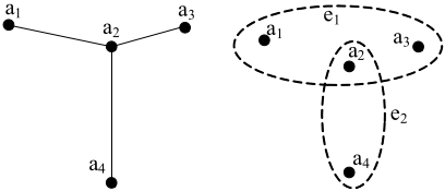
The traditional graph methods use the pair-wise relations among the training data to preserve the geometric structures of the training data. This usually is insufficient to capture the complex relations in the training data. Give an illustration on the author-paper relation in Figure 1. The left subfigure of Figure 1 uses a simple graph to describe the authorpaper relations, e.g., a1 vs. a2 (i.e., a1 and a2 are the authors of a paper), a2 vs. a3, and a2 vs. a4, but cannot imply the relations we may really focus on, e.g., the first paper has three authors (i.e., a1, a2, and a3) and the second paper has two authors (i.e., a2 and a4). The right sub-figure of Figure 1 easily indicates these two types of relations via constructing a hypergraph. Hence, this paper focuses on using a hypergraph to preserve the local structures of the training data as a hypergraph may capture more complex relations than a simple graph [Zhou et al., 2006; Somu et al., 2016; Gao et al., 2014].
By denoting a hypergraph as G = (V, E, w), where V = [vi] and E = [ei], respectively, are the set of the vertexes and the hyperedges, and w = [wi] is the weight of the hyperedges, the construction of a hypergraph includes three sequential steps: 1) the incidence matrix H representing the binary vertex-edge relation, where each element is defined as:
2) the weight vector w measuring the importance of hyperedges; and 3) the hypergraph Laplacian L, i.e., the normalized Laplacian matrix of the resulting hypergraph.
Different from the simple graph where each edge represents the vertex-to-vertex relation, the incidence matrix H of a hypergraph describes the vertex-to-hyperedge relation. To achieve this, first, given the training data X ∈ Rc×n where c and n, respectively, indicate the numbers of the features and the samples, we regard each sample as one vertex and try to generate a hyperedge for each vertex 1 by following the method in [Zhou et al., 2006]. More specifically, we generate the hyperedge ei by the following formulation:
where θ(xi, xj) indicates a similarity measurement between xi and xj (e.g., Euclidean distance on a Gaussian kernel function in this paper) and σi is the average similarity between xi and each of the other samples. Such a threshold method is very popular for the construction of the hyperedges [Somu et al., 2016; Gao et al., 2012; Peng et al., 2016a] and obviously results in that different samples have different numbers of nearest neighbors, instead of the previous methods [Elhamifar et al., 2016; Peng et al., 2016b] which set the same number of nearest neighbors to all the samples.
Second, we use the resulting incidence matrix H and the training data to learn the importance of each hyperedge, i.e., w. After this, we further obtain δ(ei) (i.e., the degree of a hyperedge ei via δ(ei) = ∑vj∈E h(vj, ei)) and d(vj) (i.e., the degree of a vertex vj via d(vj) = ∑vj∈ei,ei∈E w(ei)h(vj , ei)).
Third, we obtain the hypergraph Laplacian matrix as:
where I ∈ Rn×n is an identity matrix, De, Dv, and W, respectively, are the diagonal matrices of δ = [δ(ei)], d = [d(vj)], and w = [w(ei)].
If we want to use a hypergraph to preserve the local structures of the training data, we follow the literatures [Zhou et al., 2006; Zhang et al., 2016; Peng et al., 2017] to have the following objective function:
where ∆ = w(e)h(xi,e)h(xj,e) δ(e) and S ∈ Rc×c is the weight matrix. Obviously, Eq. (4) is equivalent to:
1 It is noteworthy that the rank of the incidence matrix H is no larger than the value of min{|V |, |E|}, where |V | and |E|, respectively, are the number of the vertexes and the hyperedges. Therefore, many previous methods set |V | = |E| for computational efficiency.
where the orthogonal constraint on the covariance matrix of X (i.e., ST XXT S = I) can be regarded to implicitly conduct subspace learning, i.e., PCA, which preserves the global structures of the training data [Morchid et al., 2014].
2.2 ProposedMethod
The three components for the construction of a hypergraph in Section 2.1 are sequential. Thus the quality of either W or L depends on H. However, H is learnt from the original training data, which usually contain redundant and irrelevant features. Thus the low-quality H is not able to output the high-quality L so that forbidding to effectively remove the noisy/redundant features via Eq. (4). In this paper, we couple the learning of the incidence matrix H with the learning of the similarity matrix S in a formulation. We expect to iteratively update each of them by fixing the others, so that they are updated adaptively to output the optimal H and S. We thus design the final objective function for our AHLFS method as follows:
whereW= diag(w) and wi is the i-th element of the vector w. Eq. (6) can directly be changed to:
where α and β are two tuning parameters, 1 is a vector whose elements are 1. The ℓ2,1-norm on S pushes to produce the row sparsity on S to select the informative features, while the constraint ST XXT S = I actually conducts subspace learning (i.e., PCA) to make the feature selection discriminative [Ang et al., 2016]. Thus the variable S is used to simultaneously select the informative features (via the sparsity constraint) and conduct subspace learning (i.e., preserving the local structures via the first term of Eq. (7) and the global structures via the orthogonal constraint) in the low-dimensional training data.
2.3 Optimization
Eq. (6) is not jointly convex to all five variables (i.e., W, S, De, Dv, and H), but is convex for each variable while fixing the others. Thus we employ the alternative optimization strategy to optimize Eq. (6), i.e., iteratively optimizing each variable while fixing the others until the algorithm converges.
Update S by fixing other variables
After fixing the other variables, the objective function with respect to S becomes:
Since the ℓ2,1-norm regularizer is convex and non-smooth, we employ the framework of iteratively reweighted least squares
(IRLS) [Wolke and Schwetlick, 1988] to optimize S, via changing Eq. (8) to:
where P is a diagonal matrix, which element is defined as:
In Eq. (9), both P and S are unknown. Moreover, P depends on S. According to the IRLS framework, we design an iterative algorithm to solve problem Eq. (9) by two sequential steps until the algorithm converges: 1) By fixing S, we obtain the P by Eq. (10); 2) By fixing P, Eq. (9) is changed to an eigen-decomposition problemwith respect to S, i.e.,
The optimal solution S in Eq. (11) is the eigenvectors of (XXT + ϵI)-1 (XLXT + βP) since XXT + ϵI is invertible, where ϵ is a very small positive value.
Update H and De by fixing other variables
According to Eq. (2) in Section 2.1, the hyperedges are generated from the original training data and thus may result in an inaccurate hypergraph. To do this, we design to learn the hyperedges from low-dimensional training data, whose redundant and irrelevant features have been removed as much as possible. Thus we use the following formulation to construct the set of the hyperedges:
where ˜σi is the average similarity between ST xi and each of other low-dimensional training data.
Eq. (12) indicates that the proposed method learns: 1) the incidence matrix H from the low-dimensional feature space; 2) different numbers of the neighbors for different samples. By contrast, both the previous simple graph methods [Nie et al., 2016; Hu et al., 2017; Zhang et al., 2017a] and the previous hypegraph methods [Somu et al., 2016; Raman et al., 2016; Zhang et al., 2017b] learn the graphs from the original data as well as assume the same number of neighbors for all the samples. Obviously, our method is more flexible and robust than the previous methods in practical applications. This may be the first work to learn a dynamic hypergraph from the low-dimensional training data for simultaneously conducting subspace learning and feature selection in a formulation.
After yielding the incidence matrix H, it is easy to work out De via the following formulation:
Update W and Dv by fixing other variables
By fixing other variables, we obtain the objective function on the variable W as follows:
| Datasets | #(Samples) | #(Features) | #(Classes) |
|---|---|---|---|
| Pcmac | 1943 | 3289 | 2 |
| Madelon | 2000 | 500 | 2 |
| Cll | 111 | 11340 | 3 |
| Yeast | 1484 | 1470 | 10 |
| Usps | 1854 | 256 | 10 |
| Mnist | 3495 | 784 | 10 |
By letting Q = D-1 e HT D- 1 2 v XSST XT D- 12 v H and q = diag(Q), according to that W is a diagonal matrix, Eq. (14) is changed to the following formulation:
We further change Eq. (15) into the following:
We use the lagrangian function to change Eq. (16) to:
where η ≥ 0 and γ ≥ 0 are the lagrangian multipliers. Based on the Karush-Kuhn-Tucker conditions, we can obtain the close-form solution for wi(i = 1, ..., n), as:
where the values of α and η are obtained in Section 2.3. After receiving w, we further obtain W = diag(w), and Dv via the following formulation:
3 Experiment Analysis
In this section, we evaluate our proposed AHLFS with the comparison methods in terms of the clustering accuracy of the clustering tasks, on eight public UCI datasets [Frank et al., 2010], whose detail is listed in Table 1.
The comparison methods include Laplacian Score (LS) [He et al., 2005], Minimize the feature Redundancy for spectral Feature Selection (MRFS) [Zhao et al., 2013], Structured Optimal Graph Feature Selection (SOGFS) [Nie et al., 2016], Coupled Dictionary Learning Feature Selection (CDLFS) [Zhu et al., 2016a], Joint Hypergraph Learning and Sparse Regression (JHLSR) [Zhang et al., 2016], and Baseline which uses all features to conduct k means clustering.
In our experiments, we set the parameters' range as {10-3 , 10-2 , ..., 103 } where all the methods can achieve their best results. We first use all the feature selection methods to select the features (i.e., {20%, 30%, ..., 80%} of all the features) and then conduct k means clustering on the selected features. We repeat k means clustering 20 times to report their average results. Finally, we employ the clustering accuracy to evaluate the clustering performance of all the methods.
3.1 Cluster Accuracy
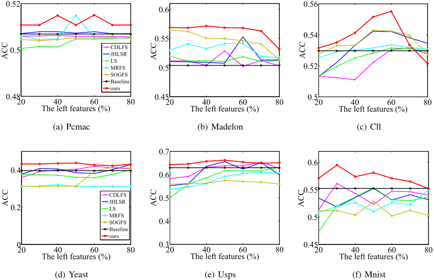
We list the clustering accuracy of all the methods with different numbers of selected features in Figure 2.
Our proposed AHLFS achieves the best clustering performance, followed by JHLSR, CDLFS, SOGFS, MRFS, LS, and Baseline. For example, our method on average improves by 6.0% and 4.9%, compared to Baseline (the worst comparison method) and JHLSR (the best comparison methods). The reason may be that our method 1) conducts subspace learning and feature selection in a framework, and 2) learns the hypergraph from the low-dimensional training data. Moreover, in the comparison methods, the methods (such as JHLSR and SOGFS) satisfying one of these benefits outperform LS which only conducts feature selection without considering any relation among the data.
In Figure 2, two observations show that there are redundant and irrelative features in the original training data and it is necessary to conduct dimensionality reduction before conducting cluster tasks. First, all the feature selection methods outperform Baseline. For example, LS (the worst feature selection method) on average improves by 3.7%, than Baseline, on all the datasets in our experiments. Second, the clustering accuracy of all feature selection methods first increases with the increase of the dimensions. After reaching to a peak, the clustering accuracy of these methods begins to decrease or even unstable. This trend indicates that a small number of the features cannot explain the samples well so that outputting bad clustering performance, while the excessively large number of the features may add redundant features to degrade the clustering performance.
3.2 Parameters Sensitivity and Convergence
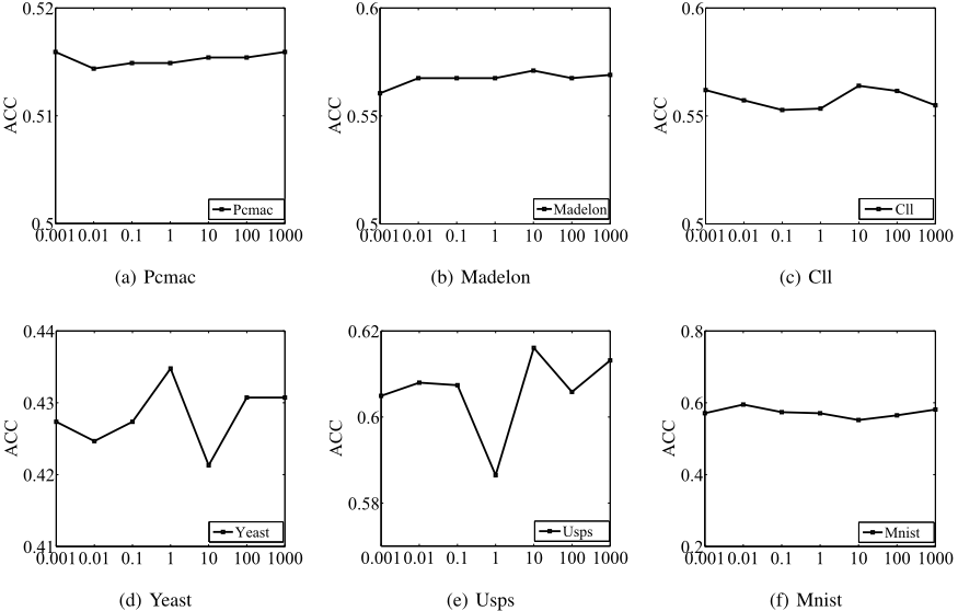
Our objective function has two tuning parameters, i.e., α and β. We fix the value of α in section 2.3. In Eq. (7), β is designed to adjust the sparsity of weight matrix S, the larger the value of β, the more the sparsity of S (i.e., the less features are selected to conduct the clustering tasks). Figure 3 demonstrates the variation of the clustering accuracy with respect to β on four datasets 2 . From Figure 3, our method achieved the best clustering performance on some values of β, which produce sparsity, i.e., selecting a subset of the features. This verified our conclusion again, i.e., it is necessary to conduct dimensionality reduction on high-dimensional data. For example, on the dataset Mnist, the best range of the values of β is [10-3 , 10-1 ], which corresponds to keep around 30% dimensions of all the features, as in Figure 2.
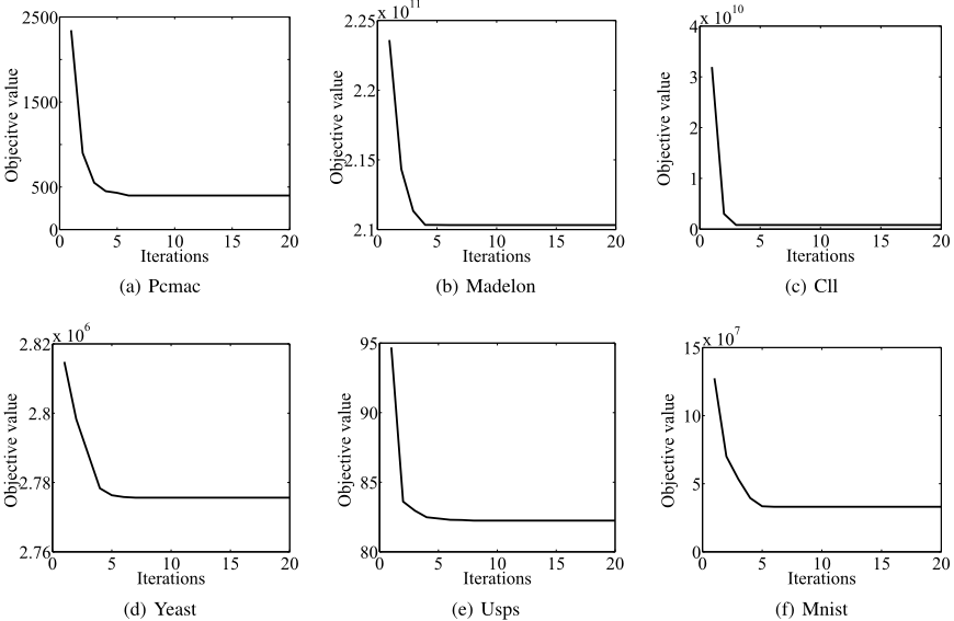
Figure 4 shows the variation of the objective values in Eq. (7), which shows that our proposed optimization method is very efficient, i.e., converging within about 10 iterations.
4 Conclusion
This paper has proposed a novel unsupervised feature selection method by coupling the hypergraph learning and feature selection in an iteration way. In this way, the hypergraph is constructed to capture the complex structures of the low-dimensional training data without the impact of redundant and irrelevant features. This makes our method reduce the feature dimensions using different methods (i.e., subspace learning and feature selection), and thus resulting in an effective and robust feature selection model. Experiment results on benchmark datasets verified the effectiveness and the robustness of the proposed method, compared to the state-of-the-art feature selection method, in terms of clustering accuracy.
2 Other datasets have similar trends for the variation of β and we did not report them due to the limited space.
Acknowledgements
This work was supported in part by the Nation Natural Science Foundation of China (Grants No: 61573270, 61363009 and 61672177), the China 973 Program (Grant No: 2013CB329404), the China Key Research Program (Grant No: 2016YFB1000905), the Guangxi Natural Science Foundation (Grant No: 2015GXNSFCB139011), the Innovation Project of Guangxi Graduate Education (YCSW2017039), the Guangxi High Institutions Program of Introducing 100 High-Level Overseas Talents, the China 1000-Plan National Distinguished Professorship, the Guangxi Collaborative Innovation Center of Multi-Source Information Integration and Intelligent Processing, and the Guangxi Bagui Teams for Innovation and Research.
@inproceedings{ijcai2017p501,
  title     = {Adaptive Hypergraph Learning for Unsupervised Feature Selection},
  author    = {Zhu, Xiaofeng and Zhu, Yonghua and Zhang, Shichao and Hu, Rongyao and He, Wei},
  booktitle = {Proceedings of the Twenty-Sixth International Joint Conference on
               Artificial Intelligence, {IJCAI-17}},
  publisher = {International Joint Conferences on Artificial Intelligence Organization},
  editor    = {Carles Sierra},
  pages     = {3581--3587},
  year      = {2017},
  month     = {8},
  note      = {Main track},
  doi       = {10.24963/ijcai.2017/501},
  url       = {https://doi.org/10.24963/ijcai.2017/501},
}
TY - CPAPER TI - Adaptive Hypergraph Learning for Unsupervised Feature Selection AU - Zhu, Xiaofeng AU - Zhu, Yonghua AU - Zhang, Shichao AU - Hu, Rongyao AU - He, Wei T2 - Proceedings of the Twenty-Sixth International Joint Conference on Artificial Intelligence, IJCAI-17 PB - International Joint Conferences on Artificial Intelligence Organization PY - 2017 SP - 3581 EP - 3587 DO - 10.24963/ijcai.2017/501 UR - https://doi.org/10.24963/ijcai.2017/501 ER -Copied
Machine-readable versions of this paper, for tools and AI agents:





