No Learner Left Behind: On the Complexity of Teaching Multiple Learners Simultaneously

1 Limitation of Classic Machine Teaching

In this section we review machine teaching and point out its limitations. We consider the problem of teaching a supervised learner, where the input space is X (e.g. Rd ) and the output space is Y (e.g. {0, 1} for classification or R for regression). Consider the set of (not necessarily i.i.d.) training sets of all sizes D = ∪∞n=0 (X × Y)n . Let Θ be the model space. A learning algorithm A is a function D ↦→ 2Θ, i.e. A takes a training set D ∈ D and maps it to a set of models. For example, the classic version-space learner Avs maps a D to Avs(D) = {θ ∈ Θ : θ consistent with D}. As another example, a soft-margin SVM learner maps D to the singleton set Asvm(D) = {ˆ θD}, where ˆ θD is the regularized empirical risk minimizer under the hinge loss.

Definition 1 (Teaching Dimension) The TD of a target model θ∗ ∈ Θ for learner A is the size of the smallest training set such that A learns θ∗ :

Here |D| is the cardinality of D. Note this is exact teaching since A must exclude all other models in Θ. If A = Avs we recover the classic TD [Goldman and Kearns, 1995]; If A = linear learners we recover the TD in [Liu et al., 2016]. TD is known for monomials, hypercubes, monotone disjunctive normal forms, linear regression, logistic regression, SVMs, etc. TD has also been extended to cooperative teacher/learner pairs [Zilles et al., 2011; Balbach, 2008].

To illustrate, 2 consider a student Aλ who runs ridge regression with regularization parameter λ > 0 on training data D = (X, Y ) with X ∈ Rn×d , Y ∈ Rn :

For any target model θ∗ ∈ Rd , θ∗ ̸= 0, the teacher can construct a single training item with X = θ∗⊤, Y = λ + ‖θ∗ ‖2 so that Aλ(D) = {θ∗ }. Therefore, TDAλ (θ∗ ) = 1, ∀θ∗ ̸= 0 [Liu et al., 2016].

Now consider a class of two students Aλ and Aλ′ , both running ridge regression but with λ ̸= λ′ . Critically, we assume that the teacher has to deliver the same lecture D to all students in the class. It is easy to see that there is no finite D that can make both students learn exactly θ∗ . Teaching dimension is not well-defined for a classroom setting.

2 Approximately Teaching a Single Student

Our plan to extend teaching dimension to a classroom setting has two steps. In this section we allow teaching to be approximate on a single student. In the next section we handle multiple students.

As the previous example shows, with multiple students but the same lecture it is generally impossible to achieve exact teaching for everyone. The teacher has to allow a certain degree of failure in some students' learned model.

Definition 2 (Student failure) Given a target model θ∗ , the student failure is a function ρ : 2Θ ↦→ R+ with the property ρ({θ∗ }) = minS⊆Θ ρ(S).

Example 1 For a ridge regression learner (1), one may define ρ(A(D)) = ‖A(D) - θ∗ ‖2 . We slightly abused the notation to use A(D) for the element in the singleton set.

Example 2 Exact teaching can be recovered by defining ρ(A(D)) = 1[A(D)̸={θ∗ }].

We say that a student A ϵ-approximately learns from lecture D if ρ(A(D)) ≤ ρ({θ∗ }) + ϵ. This allows us to extend teaching dimension to approximate teaching:

Definition 3 (Approximate Teaching Dimension) The approximate teaching dimension is the smallest training set size for the learner to ϵ-approximately learn θ∗ . Formally,

2 We will use anthropomorphic terms in the paper by calling A a student, D a lecture, and so on; we use "diversity" to mean academic diversity, i.e. differences in the learning algorithmA.

Proposition 1 The more the teacher tolerates student failure, the easier (i.e. requiring less training items) it is to teach:

Our definition of approximate TD bears a resemblance to the k-optimal teaching set in [Kobayashi and Shinohara, 2009], and can be viewed as its generalization to arbitrary learners and student failure functions. As is the case with classic TD [Goldman and Kearns, 1995], approximate TD is well-defined for all learners A : D ↦→ 2Θ but may not admit a closed-form expression. For concreteness, throughout the paper we will present two case studies: teaching conjugate Bayesian learners and ridge regression learners. We do not suggest that real-world students can be reduced to such simple learners. Nonetheless, the case studies will serve to illuminate the nuances of classroom teaching.

2.1 Case Study 1: Conjugate Bayesian Learner

The teacher wants to teach the mean µ∗ ∈ R of a Gaussian distribution N(µ∗ , σ2 ) to a student by constructing a training set D = {x1, . . . , xn}. The teacher knows the following: the student Aµ0 is a Bayesian learner with a conjugate prior µ ∼ N(µ0, σ2 0 ) on the mean; Aµ0 knows the variance σ2 ; Given D, Aµ0 performs standard Bayesian update on the mean:

The teacher measures student failure by the squared distance between the posterior mean and µ∗ , disregarding posterior variance:

Proof: If ‖µ0 - µ∗ ‖2 ≤ ϵ then there is no need to teach. Otherwise, the teacher can use a single training item:

to make ρ(Aµ0 ({x1})) = 0 by plugging it to (3). Note one teaching item is enough regardless of how far µ0 is from µ∗ . This case study can be generalized to exponential family learners [Zhu, 2013].

2.2 Case Study 2: Ridge Regression Learner

For simplicity we discuss the 1D case. The teacher wants to teach the slope θ∗ ∈ R of a linear function y = θ∗x to a student by constructing a training set D = {(x1, y1), . . . , (xn, yn)}. We further assume all training items are bounded: |x| ≤ 1. The teacher knows the following: the student performs ridge regression as in (1) with regularization parameter λ. Given D, the student estimates the parameter as

The teacher measures student failure by

Proof: If ‖θ∗ ‖2 ≤ ϵ there is no need to teach, since without teaching Aλ(∅) = {0} and this already satisfies approximate teaching. Otherwise, define

We have a constraint 0 ≤ s ≤ n due to the norm constraint on x. The teaching problem is

By inspection, one solution is n = 1, x = 1, y = θ∗ (1+λ). With this training set, Aλ({x, y}) = θ∗ and student failure ρ(Aλ({x, y})) = 0.

Both case studies will continue.

3 Teaching an Academically Diverse Class

We are now ready for the main problem of the paper. There are multiple (possibly infinite) students in a class, each with a different learning algorithm A. We denote the set of students by A. The teacher knows all students A, and must use the same lecture D to teach them. As shown earlier, exact teaching is impossible in general. The teacher's goal is then to use as few training items as possible to make sure that no student failure is too severe - i.e. to leave no learner behind.

Formally we propose a minimax formulation: The teacher seeks the minimum lecture D for all students, such that the worst student's failure is less than ϵ:

Definition 4 (Class Teaching Dimension) The class teaching dimension TDA,ϵ(θ∗ ) for all students A in class A to ϵ-approximately learn a target model θ∗ ∈ Θ w.r.t. student failure function ρ is the minimum objective of (9).

It follows that teaching a more academically diverse classroom requires no less effort.

Also the more class failure the teacher tolerates, the easier it is to teach:

For general learners the class TD can be difficult to compute, since minD is over a combinatorial space of training sets and supA involves highly nonlinear functions. We turn our attention to the two case studies, where we are able to derive a closed-form expression for TDA,ϵ. They serve to quantitatively illustrate Proposition 4, namely teaching becomes harder if the class is more inhomogeneous.

3.1 Teaching a Class in Case Study 1

We continue the story in case study 1. Now instead of a single student Aµ0 , there is a class of (possibly infinite) students A. All students know that the target distribution has the form N(·, σ2 ). They know σ2 and must infer the mean from the teacher's training data D = {x1, . . . , xn}. All students are conjugate Bayesian learners. Each student Aµi0 has a different prior on the mean µ ∼ N(µi0 , σ2 0 ), where the prior mean µi0 varies across the students but all students have the same prior variance σ2 0 . We can identify the class A = {µi0 : Aµi0 is a student} by the set of prior means. Define the lower and upper value of prior means as

The teacher knows all the above information, and must design a good lecture D to ϵ-approximately teach all students the true mean µ∗ . The teacher uses the same student failure function as in (3). We now show that the class TD is a monotonic function of µU0 - µL0 , namely the spread of students.

Lemma 1 Let a > 0 and b1 ≤ b2. We have

We omit proof for lemmas due to space, while sketching out proof outlines for theorems.

Theorem 1 The class TD of conjugate Bayesian learners is

Proof: If supµ0∈A ‖µ0 -µ∗ ‖2 ≤ ϵ then there is no need to teach, and TDA,ϵ(µ∗ ) = 0. Otherwise, TDA,ϵ(µ∗ ) ≥ 1. The training set D can be reduced to its sufficient statistics ∑ xi and n. We may write the class TD problem (9) as

Plugging in the posterior mean for Aµ0 (D) in (2), the constraint involves a quadratic form in µ0:

Since the quadratic form is convex, the supremum occurs at the boundary of A. This allows us to replace the supremum over possibly infinite students with a maximum between the two extreme students AµL0 ,AµU0 :

In other words, one of these two extreme students will have the worst student failure in the class.

We now fix n and treat ∑ xi as a free variable in R. To satisfy the constraint as much as possible, the optimal ∑ xi should minimize the LHS of (15). From Lemma 1, we have σ2 0 ∑ xi σ2 0 n+σ2 -µ∗ = σ2 σ2 0 n+σ2 -µL0 -µU0 2 . This leads to the solution

Plugging it back in (15), we have the following optimization problem:

The constraint is

Recall that we must have n ≥ 1 to teach, and n must be an integer. Taken together, the minimum n is the class TD in (12). An actual lecture D can be easily constructed from n and ∑ xi .

Theorem 1 can be interpreted as follows. The class TD of those conjugate Bayesian learners depends on class spread µU0 -µL0 , but not on how many students there are in the class. When the spread is sufficiently small, it is possible to teach the whole class successfully with a single training item. The threshold for this spread is

It is easy to see that teaching is easier as the failure tolerance ϵ increases. Teaching is also easy if the students' prior variance σ2 0 is large: in that case the students are less "stubborn" around their prior means and can be easily convinced by new evidence in data D. But when the class spread is sufficiently large, TDA,ϵ is a linear function of the spread (up to rounding). The teacher has to use more training items to teach as the class spread increases.

3.2 Teaching a Class in Case Study 2

To extend case study 2 to multiple students, let the (possibly infinite) students all be ridge regression learners as in (1) but with different regularization weights λ. Let Λ be the set of regularization weights, which is equivalent to the class A. The teacher knows Λ and must design a lecture D = {(x1, y1) . . . (xn, yn)} to ϵ-approximately teach all students in the class. Again, the teacher uses the student failure function (6).

Recall the definition of s, p in (7). The class teaching dimension problem (9) for this class can be stated as an extension of problem (8) to multiple learners:

Define

The class TD of ridge regression learners depends on these two quantities, but in a more complex manner:

Lemma 2 The student failure function ρ(Aλ(D), θ∗ ) = ( p λ+s - θ∗)2 is quasiconvex in λ.

Theorem 2 The class TD of ridge regression learners is

Proof: If ‖θ∗ ‖2 ≤ ϵ the teacher can let D = ∅. The argmin in ridge regression (1) is then determined by the regularizer. This leads to Aλ(∅) = 0, ∀λ ∈ Λ, and 0 is within ϵ of the target θ∗ by definition. Therefore, in this case the class TD is zero.

Otherwise, we must have TDΛ,ϵ ≥ 1. By Lemma 2 the supremum in constraint (20) happens at one of λL, λU due to quasi-convexity. We may replace the supremum over the whole Λ by a maximum over those two values:

Fixing n, s and applying Lemma 1 again, the optimal p denoted by p∗ (s) must happen at p∗ (s) λL+s - θ∗ = - p∗ (s) λU +s + θ∗ . This leads to p∗ (s) = 2θ∗( 1 λL+s + 1 λU +s )-1 . Plugging back this optimal value of p the teaching problem becomes

By inspection the (real-valued) solution is

The class TD is obtained by n ≥ 1 and rounding. An optimal training set can be constructed from n, s, p. Again, the class TD depends on the class spread λU -λL, not the number of students. As the class spread becomes wider, the class TD increases at a rate of (λU - λL)/(2√ϵ).

4 Optimal Class Partitioning

The previous section highlights Proposition 4, namely it is hard to teach an academically diverse class. The root of the problem is the classroom setting, where the teacher must use the same lecture D on all students. We now consider a setting where the teacher is allowed to partition the class into sections, and different sections may use different lectures. This is a familiar tradeoff in reality: Parents want smaller class sizes, but schools need to control expenses. One extreme partition is to have each student in their own section, i.e., personalized education. But this may not be optimal in the teacher's effort to deliver lectures: presumable very similar students should share the same lecture. We now show that there is a sweet spot, such that the aggregate training set size is minimized while guaranteeing no learner left behind.

We formulate the optimal class partition problem as follows. For a class A we use π = π(A) to denote a partition, i.e. a set of sections: ∅ /∈ π; ∪S∈πS = A; ∀S, S′ ∈ π, S ̸= S′ ⇒ S ∩ S′ = ∅. Each section S ∈ π is now a smaller class. To ϵ-approximately teach all students in S, by definition the teacher needs TDS,ϵ(θ∗ ) training items. Define the aggregate training set size under π as n(π) ≡ ∑S∈π TDS,ϵ(θ∗ ). This implies that the teaching effort is the accumulative teaching time over all sections, where each training item takes unit time. Note n(π) is not the number of unique training items across all sections.

Definition 5 The partition teaching dimension is defined as

where the optimal class partition π∗ is the one that achieves the minimum.

Our two case studies, continued below, demonstrates that there are nontrivial class partition sweet spots.

4.1 The Optimal Class Partition in Case Study 1

Recall the class A consists of students with different prior distributions N(µ0, σ2 0 ), where µ0 is bounded between µL0 and µU0 . We first note that, unlike the class TD which only depends on the spread µU0 - µL0 , the optimal partition also depends on the topology of A. For example, when all students form two degenerate (elements overlapping) clusters at the two extrema µL0 and µU0 , the teacher can partition the class into two sections by the clusters. Each section would require at most one training item per Theorem 1, leading to a partition TD of at most two. In contrast, the partition TD is very different when the class is dense in the interval A = [µL0 , µU0 ], which is our focus below.

Let cl(·) be the closure of a set (for example, cl([0, 1)) = [0, 1]), and conv(·) be the convex hull of a set.

Lemma 3 Given any A ⊂ R, we have the class TD

Lemma 4 For a bounded A ⊂ R, one optimal partition π∗ where A = ∪TDπ∗,ϵ(·)) i=1 Ai as in (26) must satisfy

1. All conv(Ai)'s are disjoint;
2. Any Ai can be taught by 1 item, that is, the class TDAi,ϵ(·) = 1.

Theorem 3 For A = [µL0 , µU0 ] satisfying supµ∈A ‖µ - µ∗ ‖2 > ϵ, an optimal partitioning π∗ is to break A into intervals each of length defined by the RHS of (19), where each section can be taught with a single teaching item. The corresponding partition teaching dimension is

Proof: From Lemma 4, we know that one optimal partition should be in the form of A = ∪TDπ∗,ϵ i=1 Ai with Ai = [µi-1 , µi ] where µ0 = µL0 and µTDπ∗,ϵ = µU0 . Given such partition structure, we can apply the greedy procedure to find one optimal partition: start from µ0 and maximize µ1

for A1 given TDA1,ϵ = 1, then maximize µ2 for A2 given TDA2,ϵ = 1, and so on until that µi exceeds µU0 . From Theorem 1, the largest range of students µi -µi-1 that one training item can teach satisfies:

(Note that the "0" teaching case is excluded automatically because supµ∈A ‖µ - µ∗ ‖2 > ϵ). It implies that the largest range is µi - µi-1 ≤ 2√ϵ ( σ2 0 σ2 +1), precisely (19). Thus the minimal number of sections is given by (27).

Comparing the partition TD in (27) to the whole class TD in (12), we see that class partition is especially helpful when σ2 0 → 0, i.e. when the students are stubborn. Stubborn students blow up the whole class TD, but having them in different sections prevents the blow up due to the added 1 in the denominator.

4.2 The Optimal Class Partition in Case Study 2

For simplicity, we consider a class consisting of students dense in the interval A ≡ Λ = [λL, λU ]. If |θ∗ | ≤ √ϵ then trivially TDπ,ϵ(θ∗ ) = 0. We only consider the nontrivial case |θ∗ | > √ϵ below.

Theorem 4 For a class A = [λL, λU ] and |θ∗ | > √ϵ, let a = 2 ( |θ∗ | √ϵ -1)-1 . The partition teaching dimension is

Proof: (sketch) It can be shown that each section should be an interval of students; Moreover, if one interval of students can be taught by n training items, then it can be partitioned into two intervals such that one can be taught by n-1 items, and the other can be taught by 1 item. These imply that an optimal class partition divides Λ at λL = λ0, λ1, . . . , λn-1 < λU , λn ≥ λU , such that each section (except the last one) is maximal while still can be ϵ-approximately taught with one training item. Then π∗ = {[λi-1, λi] : i = 1 . . . n} and TDπ∗ ,ϵ(θ∗ ) = n.

To find out the values of λi and n, we identify those maximal sections. Starting from λL = λ0 and applying (22), the maximum λ1 must satisfy λ1-λ0 2√ϵ |θ∗ |- λ0+λ1 2 = 1. This leads to λ1 = a + (1 + a)λ0 and more generally λt = a + (1 + a)λt-1. Note the intervals increase with t, which is different from the equal partitions in case study 1. Let zt = λt + 1 then the above series becomes zt = (1+a)zt-1 = (1+a)t z0, hence λt = (1+a)t (λL +1)-1. The value n is the smallest t such that λt ≥ λU , namely t ≥ log(1+a) ( λU +1 λL+1 ). Rounding completes the proof. Compared to the class TD which is O(λU - λL), the partition TD is always better.

4.3 A Simulation for Illustration

We illustrate in Figure 1 the benefit of teaching an optimally partitioned class with a simulation for case study 2. There are 1000 ridge regression students (1) with λL = 10-1 , λU =

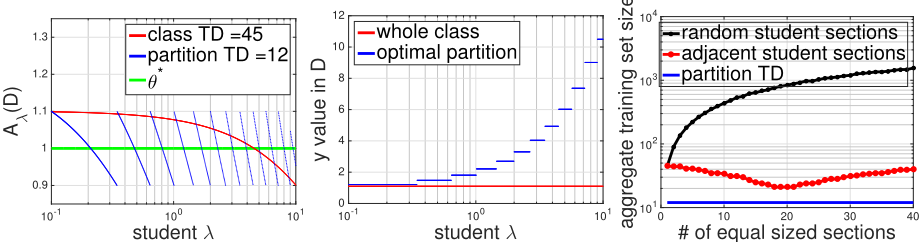
101 and the students are evenly spaced in log(λ). The students form the class A (or Λ), and they are the x-axis in Figure 1. The teacher wants to ϵ-approximately teach the target model θ∗ = 1, with ϵ = 0.01.

The left panel shows what model each student learned. The green curve simply marks the target model θ∗ . The red curve shows the effect of teaching the whole class A with the optimal "whole-class lecture" D as defined in Theorem 2 proof. The class TDA,0.01(1) = 45. The teacher needs 45 training items in D to guarantee ϵ-learning for everyone. Since we defined student failure as the squared difference (6), the students succeed if they learn a model Aλ(D) within ±√ϵ = ±0.1 of θ∗ . This is precisely what the red curve shows. In contrast, the blue curves show the optimal partition as in Theorem 4 proof. Each blue segment represents a section that can be ϵ-taught with one training item. Indeed each section of the learned models are within θ∗ ± 0.1. There are 12 sections in the optimal partition: TDπ∗ ,0.01(1) = 12.

The center panel shows the lectures D. In all D, we have the construction x = 1 always, while y and multiplicity differ. The curves should be read as follows: the value y at a student λ means that the student is sharing a lecture which contains the training point (x = 1, y). The red curve gives y = 1.101 for the "whole class lecture," which means that D consists of 45 identical instances of the point (1, 1.101). The blue curve segments are for the 12 sections of the class, each section's D has a single instance. For example, the right-most section has D = {(1, 10.496)}. Note how the teacher increases y for sections with larger λ's to account for regularization.

The right panel shows the aggregate training set size n(π) needed to teach various non-optimal class partitions π. We simply divide the 1000 students into equal-sized sections, where the number of sections is on the x-axis. The red curve shows the case where students with adjacent λ values are partitioned together. When the number of sections is 1, the aggregate training set size is 45 as we mentioned earlier (it is bad to teach a large class). When the number of sections is 1000 (not shown), that size is trivially 1000 (it is inefficient to perform fully personalized education). Note the minimum happens at around 20 - not 12 - sections. And the minimum aggregate size is 21, larger than the partition TD of 12 indicated by the blue line (simply dividing the class evenly into sections does not quite work). This highlights the importance of intelligent uneven partitions computed by machine teaching (center panel) to achieve optimality. Finally, the black curve shows the case where the students are randomly assigned to each section. This is a bad idea as each section now takes about the same training set size to teach as the whole original class! Under our setting it is important to keep the sections homogeneous.

5 Discussions

Readers familiar with Probably Approximately Correct (PAC) learning and VC theory may wonder how our work relates to those framework. The class TD in Definition 4 provides a good contrast. We are controlling the error to be uniformly below ϵ. But a major difference is that we do not rely on concentration of measure over i.i.d. samples in the training set. Instead, we start with the target concept θ∗ and then optimize the training set D. Therefore, we do not have the "P" in PAC learning. In terms of VC dimension, it is known that VC and TD are distinct measures [Goldman and Kearns, 1995], and the distinction carries over to our classroom teaching setting.

In order to make analysis tractable, we made several simplifying assumptions that should be relaxed in future work. A strong assumption is that the teacher knows everything about the students A (i.e., their learning algorithms). Future work may allow the teacher to probe the students if this is not the case, and jointly optimize the effort of teaching and probing.

A variant that is ethically questionable but unfortunately occurs in practice is for a teacher to give up on at most δ fraction of the students, to allow them to have arbitrarily large student failures. The remaining students must ϵ-approximately learn. This type of (ϵ, δ) class TD can be much smaller.

Interestingly, in the education literature it was suggested that some cultures prefer large classes, with the argument that students can observe and learn from each other's mistakes [Stigler and Hiebert, 1998]. It is possible to build this into machine teaching theory by formulating the class A as a multi-agent system. More research is needed to understand how academic diversity benefits teaching.

In summary, this paper advances machine teaching theory and provides a potential theoretical framework for optimizing real-world education resource allocation in the future.