
Multi-Positive and Unlabeled Learning
Proceedings of the Twenty-Sixth International Joint Conference on Artificial Intelligence. Main track. Pages 3182-3188.
https://doi.org/10.24963/ijcai.2017/444
Keywords
- Machine Learning: Machine Learning
- Machine Learning: Semi-Supervised Learning
- Machine Learning: Classification
Abstract
The positive and unlabeled (PU) learning problem focuses on learning a classifier from positive and unlabeled data. Some methods have been developed to solve the PU learning problem. However, they are often limited in practical applications, since only binary classes are involved and cannot easily be adapted to multi-class data. Here we propose a one-step method that directly enables multi-class model to be trained using the given input multi-class data and that predicts the label based on the model decision. Specifically, we construct different convex loss functions for labeled and unlabeled data to learn a discriminant function F. The theoretical analysis on the generalization error bound shows that it is no worse than k√k times of the fully supervised multi-class classification methods when the size of the data in k classes is of the same order. Finally, our experimental results demonstrate the significance and effectiveness of the proposed algorithm in synthetic and real-world datasets.
- [Blanchard et al., 2010] Gilles Blanchard, Gyemin Lee, and Clayton Scott. Semi-supervised novelty detection. The Journal of Machine Learning Research, 11:2973-3009, 2010.
- [du Plessis et al., 2014] Marthinus C du Plessis, Gang Niu, and Masashi Sugiyama. Analysis of learning from positive and unlabeled data. In Advances in Neural Information Processing Systems, pages 703-711, 2014.
- [Elkan and Noto, 2008] Charles Elkan and Keith Noto. Learning classifiers from only positive and unlabeled da- ta. In Proceedings of the 14th ACM SIGKDD internation- al conference on Knowledge discovery and data mining, pages 213-220. ACM, 2008.
- [Fung et al., 2006] Gabriel Pui Cheong Fung, Jeffrey X Yu, Hongjun Lu, and Philip S Yu. Text classification without negative examples revisit. Knowledge and Data Engineer- ing, IEEE Transactions on, 18(1):6-20, 2006.
- [Kanoun et al., 2011] Slim Kanoun, Adel M Alimi, and Yves Lecourtier. Natural language morphology integra- tion in off-line arabic optical text recognition. Systems, Man, and Cybernetics, Part B: Cybernetics, IEEE Trans- actions on, 41(2):579-590, 2011.
- [Latulippe et al., 2013] Maxime Latulippe, Alexandre Drouin, Philippe Giguere, and Franc ¸ois Laviolette. Accelerated robust point cloud registration in natural environments through positive and unlabeled learning. In Proceedings of the Twenty-Third international joint conference on Artificial Intelligence, pages 2480-2487. AAAI Press, 2013. IJCAI
- [Li et al., 2011] Wenkai Li, Qinghua Guo, and Charles Elka- n. A positive and unlabeled learning algorithm for one- class classification of remote-sensing data. Geoscience and Remote Sensing, IEEE Transactions on, 49(2):717- 725, 2011.
- [Li et al., 2014] Sheng Li, Ming Shao, and Yun Fu. Local- ity linear fitting one-class svm with low-rank constraints for outlier detection. In Neural Networks (IJCNN), 2014 International Joint Conference on, pages 676-683. IEEE, 2014.
- [Liu and Tao, 2016] Tongliang Liu and Dacheng Tao. Clas- sification with noisy labels by importance reweighting. IEEE Transactions on pattern analysis and machine in- telligence, 38(3):447-461, 2016.
- [Liu et al., 2003] Bing Liu, Yang Dai, Xiaoli Li, Wee Sun Lee, and Philip S Yu. Building text classifiers using posi- tive and unlabeled examples. In Data Mining, 2003. ICD- M 2003. Third IEEE International Conference on, pages 179-186. IEEE, 2003.
- [Liu et al., 2017] Tongliang Liu, Dacheng Tao, Mingli Song, and Stephen J Maybank. Algorithm-dependent generaliza- tion bounds for multi-task learning. IEEE transactions on pattern analysis and machine intelligence, 39(2):227-241, 2017.
- [Mohri et al., 2012] Mehryar Mohri, Afshin Rostamizadeh, and Ameet Talwalkar. Foundations of machine learning. MIT press, 2012.
- [Nguyen et al., 2011] Minh Nhut Nguyen, Xiaoli-Li Li, and See-Kiong Ng. Positive unlabeled leaning for time se- ries classification. In IJCAI, volume 11, pages 1421-1426. IJCAI
- [Plessis et al., 2015] Marthinus D Plessis, Gang Niu, and Masashi Sugiyama. Convex formulation for learning from positive and unlabeled data. In Proceedings of the 32nd In- ternational Conference on Machine Learning (ICML-15), pages 1386-1394, 2015.
- [Saberian and Vasconcelos, 2011] Mohammad J Saberian and Nuno Vasconcelos. Multiclass boosting: Theory and algorithms. In Advances in Neural Information Processing Systems, pages 2124-2132, 2011.
- [Schwenker and Trentin, 2014] Friedhelm Schwenker and Edmondo Trentin. Pattern classification and clustering: a review of partially supervised learning approaches. Pat- tern Recognition Letters, 37:4-14, 2014.
- [Tsochantaridis et al., 2004] Ioannis Tsochantaridis, Thomas Hofmann, Thorsten Joachims, and Yasemin Altun. Support vector machine learning for interde- pendent and structured output spaces. In Proceedings of the twenty-first international conference on Machine learning, page 104. ACM, 2004.
- [Yang et al., 2014] Peng Yang, Xiaoli Li, Hon-Nian Chua, Chee-Keong Kwoh, and See-Kiong Ng. Ensemble positive unlabeled learning for disease gene identification. 2014.
- [Yu, 2003] Hwanjo Yu. Svmc: Single-class classification with support vector machines. In IJCAI, pages 567-574. IJCAI
References were extracted automatically from the PDF and may contain errors.
Full text extracted automatically from the PDF; figures, tables and equations may differ. The PDF is the version of record.
1 Introduction
Training examples are labeled as positive or negative in the conventional binary classification problem. In contrast, the positive and unlabeled (PU) learning problem aims to learn a classifier from positive and unlabeled data, where unlabeled data contain both positive and negative examples. Many realworld applications can be generalized as PU learning problems. For example, when distinguishing urban areas and nonurban areas using remote-sensing data [Li et al., 2011], urban examples can easily be labeled whereas non-urban examples are too diverse to be fully labeled. In gene association studies [Yang et al., 2014], confirmed causative genes of various human diseases are considered positive while all other unknown genes are treated as unlabeled data. In security systems, authorised user upload a series of photographs of his own face while any picture of a person in front of the camera is regarded as unlabeled. Some classical applications such as text classification [Fung et al., 2006; Kanoun et al., 2011] and information retrieval [Latulippe et al., 2013; Schwenker and Trentin, 2014; Yu, 2003; Nguyen et al., 2011;
Li et al., 2014; Liu et al., 2017] can also be regarded as PU learning problems.
Some effective algorithms have been developed to solve the PU learning problem. Biased support vector machine (Biased SVM) solves the PU problem by treating unlabeled data as negative data with noise [Liu and Tao, 2016] and using a cost-sensitive SVM to generate the classifier [Liu et al., 2003]. [Elkan and Noto, 2008] showed that the probability predicted by a classifier trained on positive and unlabeled examples has a constant difference from the true conditional probability. The resulting classifier can thus be constructed by first training an initial classifier using traditional supervised learning methods on positive and unlabeled data and then estimating the constant difference based on positive data. [du Plessis et al., 2014] proved that convex loss functions are inapplicable to learning PU problem classifiers, due to the systematic estimation bias, and instead recommended nonconvex loss functions, e.g. ramp loss, for PU learning. [Plessis et al., 2015] then demonstrated that employing different convex loss functions over positive examples and unlabeled examples overcomes the difficulty in optimizing non-convex loss functions in [du Plessis et al., 2014] while guaranteeing learning performance.
Although existing PU learning algorithms are effective and show promising performance in a number of different applications, they share the limitation that only binary classes are involved. Hence, they are not easy to adapt to the multi-class data which is common in real-world applications. For example, more than one person might be authorized by the security system, thus their face images are grouped into distinct positive classes. A personalized email filter should allow some spam to pass through the system in addition to non-spam emails, which are also organized into several positive classes.
Here we study the Multi-Positive and Unlabeled learning (MPU) problem, in which labeled data from multiple positive classes and unlabeled data from either the positive classes or an unknown negative class are provided for learning. We aim to construct different convex loss functions for labeled and unlabeled data to eliminate the systematic estimation bias. We achieve this by learning a discriminant function F : X × Z → R over the input and the encoded output pairs (x1, z1), · · ·, (xn, zn) ∈ X × Z, with the new output space Z generated by encoding the original output space Y. We provide a theoretical analysis of the generalization error bound of MPU, which is no worse than k√k times of the fully supervised multi-class classification methods when the size of the data in different classes is of the same order. Finally, our experiments over synthetic and real-world MPU datasets demonstrate the practical significance of studying classification problems involving multiple positive data from different classes and unlabeled data.
2 ProblemFormulation
Supposing the data are from k classes, the first k - 1 classes are regarded as positive while the k-th class is negative. In the MPU problem of interest, we assume that the labeled data are sampled from k - 1 positive classes and the unlabeled data could be from either positive classes or a negative class. Given a training set:
where nl and nu represent the number of labeled and unlabeled samples respectively, and xi ∈ X ⊆ Rd , yi ∈ Y = {1, 2, ..., k}, MPU aims to learn a decision function f : X → Y based on the training data.
2.1 Multi-Positive and Unlabeled Learning
In classical multi-class classification, given the class prior πi = p(y = i), i = 1, 2, ..., k, we can learn the classifier based on the decision function f(x) by minimizing the expected misclassification rate:
where ∑ki=1 πi = 1. Ri(f) = Pi(f(x) ̸= i) denotes the expected misclassification rate on the i-th class, and Pi is the marginal probability. By learning a discriminant function F : X × Y → R which can be treated as the reliability or the score of the prediction over input/output pairs, we can derive the prediction by maximizing F given some input x [Tsochantaridis et al., 2004]. Therefore, the decision function f can be expressed as:
where W is the parameter matrix. For simplicity, we define F(x, y) = F(x, y;W) in the following paragraph.
In the MPU problem, the unlabeled samples is a mixture of samples in k classes, therefore the distribution of unlabeled data can be denoted by a linear combination of the distribution of the samples in k classes. Defining PX as the marginal probability of unlabeled data:
where πi is the unknown class prior which can be estimated with the method in [Blanchard et al., 2010]. Note that we have assumed that the k-th class is negative, then there are no labeled data in the k-th class. R(f) must, therefore, be reformulated to exclude Rk(f). We introduce RX(f) to denote the probability that the unlabeled sample has not been classified as the k-th class:
Note that Rk(f) can be expressed with RX(f), and the distribution of the unlabeled data can be easily obtained from the input data. Hence, applying Eq.(5) to Eq.(2) and note that ∑ki=1 πi = 1, the expected misclassification rate R(f) can be written as:
in which Pi(f(X) ̸= k) represents the probability that the sample in the i-th class has not been classified as the k-th class. Note that Ri(f) (RX(f)) can be treated as the probability that the sample in the i-th class (in the unlabeled data) has not been classified as the i-th (k-th) class. Therefore, each term of the expected misclassification rate R(f) can be expressed as:
in which i is the true label of the sample (which is unknown for unlabeled data). The left hand side of Eq.(7) is the rate that the sample in the i-th class has not been classified as the j-th class, which can be decomposed as the summation of k - 1 terms, each of which represents the rate of classifying the sample in the i-th class to the m-th class.
Based on the analysis above, denoting F(x(i) , f(x) = j) as the prediction score of the sample in the i-th class which is classified as the j-th class, the empirical loss of the sample can be defined as:
in which F(x(i) , f(x) ̸= j) means the empirical loss that the sample in the i-th class has not been classified as the j-th class. And l(F (x(i) , f(x) = m)) is the loss of misclassifying a sample from the i-th class into the m-th class. Note that the loss in Eq.(8) is computed on k-1 classes since each term of the expected misclassification rate R(f ) is computed on k-1 classes according to Eq.(7).
Therefore, given Eq.(8), the loss function can be expressed based on Eq.(6):
in which ˜ y is some unknown label of the unlabeled data, and the last equation is derived from Eq.(8) since there are k - 2 same terms between two L(·)'s and only two l(·)'s are remained after subtraction.
Since adopting the same convex loss function for positive and unlabeled data can lead to systematic estimation bias which causes an incorrect classification boundary [du Plessis et al., 2014], it is appropriate to use distinct loss functions over labeled and unlabeled data. For efficiency, it is better that both loss functions are convex. Therefore, we define:
It is worth noting that the hinge loss is appropriate here to get a convex model because when the sample is correctly labeled, the loss proposed in Eq.(10) is a fixed value (l(F(x(i) , f(x) = i)) = 1/2). Therefore, both l(·) and L(·) in Eq.(11) and the model (Eq.(11)) are convex.
2.2 Discriminant Function Construction
To specify Eq.(11), we need to construct the discriminant function F (x, f (x); W).
To handle multiple classes effectively, we encode class labels using vectors (z1, z2, ..., zk) ∈ Rr , where r indicates the length of the code and zi is the codeword of the i-th class. Given the parameter matrix Wr×d (in which d is the dimension of the input space), we define:
In Eq.(12), the original input space X is mapped into Z, and the geometric result of the inner product is the projection value of the input data to the codeword zj, which can be treated as the score on the j-th class. The decision function can be expressed as Eq.(3).
Note that in order to achieve an effective result, the prediction score of x(i) on the i-th class should be the largest one, and the margins between the scores of x(i) on different classes should be large enough. The following optimization problem is a possible approach to encode y by maximizing the margins between the codewords:
in which the length of the codewords is fixed as r = k - 1. It has been proved in [Saberian and Vasconcelos, 2011] that the vertices of a k - 1 dimensional regular simplex centered at the origin are the solutions of Eq.(13).
Assuming that there are ni labeled samples belonging to the i-th class, i = 1, 2, · · ·, k - 1, and nu samples are unlabeled. Applying Eq.(12) to Eq.(11), the empirical loss function can be written as:
where x(i) j denotes the j-th sample in the i-th class and x(˜ yj′ ) j ′ denotes the j ′ -th sample which is unlabeled, whose true label is ˜ yj ′ which is unknown. The first term is the regularization term, and [x]+ = max(x, 0).
Note that the parameter matrix W is the only parameter needing to be optimized in the first term on the right hand side of Eq.(14). In the second term, however, since the input data are unlabeled, we also need to optimize z˜ yj′ , which is the encoded result of the true class of the unlabeled data. Therefore, defining ˜y = (˜ y1, ˜ y2, ..., ˜ ynu ) (where ˜ yi ∈ {1, 2, ..., k}), there are two parameters W and ˜y needing to be optimized.
2.3 Optimization of Problem (Eq.(14))
Giving the empirical loss function Eq.(14), there are two parameter matrices in the loss function that need to be optimized, where W is the parameter matrix in the discriminant function Eq.(12) and ˜y denotes the true labels of the unlabeled samples. The proposed optimization function Eq.(14) is non-convex. However, fixing one of the variables, and the problem becomes convex w.r.t. the other one. Thus, we propose an optimization algorithm by fixing one of the variables alternatively until the optimization function converges. The details are given by the pseudo-code in Algorithm 1.
Algorithm 1 Multi-positive and unlabeled learning
Input: Number of classes k, dataset T = {(xl, yl)}nl l=1 ∪ {(xu)}nu u=1 , encoded matrix Z.
Initialization: setW←W0, ˜y ← ˜y0.
repeat
- FixedW, update ˜y that minimize ˆ J(W, ˜y)
for i = 1 to nu do
for c = 1 to k do
J(W, ˜y|˜
Compute ˆ
end for
j = argmin
˜
yi = j
end for
- Fixed ˜y, update W that minimize ˆ J(W, ˜y)
until converge
Output: parameter matrixW
3 Theoretical Analysis
In this section, we provide the theoretical analysis of the generalization error bounds of the proposed method. The proofs are shown in Appendix A∼Appendix C.
Firstly, substitute a generalized form for Eq.(10):
For a given dataset, there is an upper bound D, that makes 0 ≤ ˆlρ ≤ D. Without loss of generality, scaling lρ which makes ˆlρ ∈ [0, 1], the normalized loss lρ is defined as:
c
ˆ
yi = c)
J(W, ˜y|˜
yi = c)
and Eq.(8) becomes:
so Eq.(11) can be rewritten as:
where the first term represents the loss of the labeled positive data and the second term represents the loss of the unlabeled data.
In the following paragraph, we show the generalization error bounds of the two terms in Eq.(17) in Theorem 2 and 3 respectively. We begin with the first term, and the constant 12 is ignored for simplicity.
Theorem 1. Let hj(x(i) ) = F(x(i) , f(x) = j) ∈ Hi ⊆ RX×Y where Hi is a hypothesis set with Y = 1, 2, ..., k. Fix ρ > 0. For any 0 < δ < 1, with probability at least 1-δ, the generalization bound holds for all hi ∈ Hi:
Theorem 2 presents the error bound for labeled data from each positive class, so we can summarize them to get the error bound of the first term in Eq.(17).
Note that it is difficult to get the error bound of the second term in Eq.(17), so we aim to decompose it into two terms using the following lemma.
Lemma 1. Define
the last term of Eq.(17) can be decomposed as follows:
where π∗ c := p(y = c) is the true class prior of the c-th class.
Based on the decomposition result from Lemma 1, the generalization error bound of the second term in Eq.(17) can be obtained by bounding each term in Eq.(19) (see Appendix C for detail). The result is shown in the following theorem:
Theorem 2. Fix ρ > 0. For any 0 < δ < 1, with probability at least 1-δ over the samples in N = N1 ∪· · ·∪Nk-1 ∪Nu, the generalization bound holds for all hi ∈ Hi:
Summarizing the inequality in Theorem 2 and 3, we get the generalization error bound of Eq.(17), and the order of the error bound is shown below:
Theorem 3. As ni → ∞, i = 1, 2, ..., k - 1; nu → ∞ and k →∞, the generalization error bound of the proposed method is of order:
Note that for fully labeled data, the samples are i.i.d., and the generalization error bound would be of order O(k2 /√n1 + · · · +nk-1 +nu). The proposed method is, therefore, no worse than k√k times of the fully supervised multi-class classification methods when the size of the data in different classes is of the same order.
4 Experiments
We conducted two sets of experiments: a toy experiment to qualitatively show the properties of the proposed algorithm, and a quantitative evaluation of the algorithm on real-world datasets. The new MPU algorithm was compared with the binary PU learning methods (BPU) such as BPU(DH) method in [Plessis et al., 2015] which created a double hinge loss function for the unlabeled data, BPU(ramp) method in [du Plessis et al., 2014] where the non-convex ramp loss was used, and biased SVM method [Liu et al., 2003]. All binary methods were generalized to solve the multi-class problem with one-versus-all method.
4.1 Experiment on Toy Data
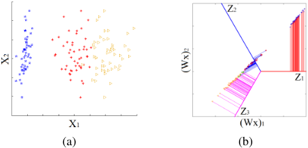
We first conducted an experiment on the IRIS dataset from the UCI repository. There are 3 classes in the dataset with 50 samples for each. The first two classes were treated as positive and the third class as negative. For the simplicity of illustration, we reduced the dimensionality to 2 via principal component analysis, with 50 labeled data samples (25 in class 1 and 25 in class 2) and 100 unlabeled data samples drawn (Fig.1 (a)). The examples were projected into space Z and the classification result is shown in Fig.1 (b).
The three lines represent the codeword zi, while the three classes of mapped input data are shown in different colors (the misclassified points are in green). Each point was projected to the three codewords (only one projection is drawn for simplicity). The projection value of input data to zi represents the score on the i-th class. The label of the class with the maximum score was assigned to the input data. Nearly all of the data was classified correctly.
| Dataset | examples | variables | classes |
|---|---|---|---|
| Image Segment | 2310 | 19 | 7 |
| Letter | 20000 | 16 | 26 |
| USPS | 11000 | 256 | 10 |
| MNIST | 70000 | 784 | 10 |
4.2 Real-world Data Set
Experiments were conducted on four different datasets, and the relevant metadata for each dataset are shown in Table 1.
The conventional methods for the binary PU learning problem were generalized to solve the MPU learning problem with one-versus-all method and were compared with the new MPU algorithm in terms of classification accuracy and training time. All datasets were preprocessed, with half of the samples in each positive class regarded as labeled, while the other half together with all the samples in the negative class regarded as unlabeled. The class priors were assumed to be known at the time of training 1 . Furthermore, the fully labeled datasets trained with linear SVM were compared with all the methods mentioned above.
Classification accuracies are shown in Table 2 (All methods use linear kernal). The proposed MPU algorithm achieves the best result of all the PU learning methods and is comparable to the linear SVMmethod trained on fully labeled data, since our one-step method allows direct model to be trained using the given input data and obtains the label based on all the model decisions, while the generalized BPU methods share the disadvantage such as error accumulation that oneversus-all method has.
The binary PU learning results are shown in Table 3. The seventh class was fixed as the negative class, while the other classes were treated as positive class. One of the positive class was chosen at a time, and half of the examples in the chosen positive class were labeled while the other half together with the negative examples were unlabeled. Our proposed method shows comparable performance on the binary PU learning problem with other BPU methods in terms of classification accuracy.
1 The class priors can be estimated with the methods in [Blanchard et al., 2010] in practice.
| Method | Image Segment | Letter | USPS | MNIST |
|---|---|---|---|---|
| Linear SVM | 93.51 | 84.05 | 96.32 | 93.61 |
| MPU | 90.26 | 70.12 | 92.86 | 90.78 |
| BPU(DH) | 88.31 | 62.98 | 89.13 | 86.92 |
| BPU(Ramp) | 88.74 | 63.18 | 89.94 | 87.04 |
| Biased-SVM | 85.93 | 45.27 | 87.14 | 84.98 |
| Dataset | MPU | BPU(DH) | BPU(Ramp) | Biased SVM |
|---|---|---|---|---|
| Class 1vs7 | 0.15 | 0.61 | 0.45 | 0.30 |
| Class 2vs7 | 2.73 | 3.18 | 3.18 | 2.88 |
| Class 3vs7 | 3.64 | 3.79 | 3.48 | 4.55 |
| Class 4vs7 | 1.06 | 1.66 | 1.67 | 1.97 |
| Class 5vs7 | 0.45 | 0.76 | 0.61 | 0.61 |
| Class 6vs7 | 0.61 | 0.76 | 0.61 | 0.45 |
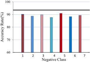
Next, we illustrate the robustness of our proposed methods on the choice of the negative class. Fig.2 shows the classification accuracies for choosing different classes as the negative class. The black line represents the accuracy of the method training on a fully labeled dataset. It is shown that the fluctuate of the classification accuracy is small when choosing different classes as the negative class. Thus our proposed methods is robust on the choice of the negative class.
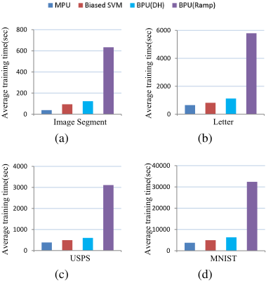
The training time on six datasets given in Fig.3 show that the MPU algorithm is faster than other generalized binary PU methods on large datasets, since the one-versus-all method needs to train k classifiers with all samples in the datasets.
5 Conclusion
This paper presents the MPU algorithm for solving the multipositive and unlabeled learning problem. We show that the MPU algorithm allows direct model to be trained with respect to the multi-class input data rather than via a two-step approach which often leads to a high classification error rate. The theoretical analysis shows that the generalization error bounds of the MPU algorithm are comparable to k√k times of fully supervised multi-class classification methods when the size of the data in different classes is of the same order. Experimentally, the proposed MPU algorithm outperforms current state-of-the-art methods in the MPU problem and is as accurate in the BPU problem with a less computational burden. Moreover, our method is comparable to the methods training using fully labeled data and robustly chooses the negative class.
A Proof of Theorem 1
Based on the definitions 3.1 and 3.2 in [Mohri et al., 2012], given Ni = (x(i) 1 , ..., x(i) ni ), i = 1, 2, ..., k - 1;Nu = (x1, ..., xnu ); N = N1∪···∪Nk-1∪Nu, define the empirical Rademacher complexity of Hi with respect to the sample Ni:
where σ = (σ1, ..., σni )⊤ and σi ∈ {-1,+1}. Denote by Rni (Hi) the Rademacher complexity w.r.t. p(x|y = i), and Rnu (H) the Rademacher complexity w.r.t. p(x, then we have:
We then have (Proposition 8.1 in [Mohri et al., 2012]):
where α = supx∈Rd √k(x, x) with k(·, ·) be a PDS kernel and β = sup(||w||) for some β ≥ 0.
Define G = max{h1, h2, ..., hk}, then the empirical Rademacher complexity of G can be upper bounded by (Lemma 8.1 in [Mohri et al., 2012]):
Applying Eq.(25) to Theorem 8.1 in [Mohri et al., 2012], and note that the Lipschitz constant of lρ is 1 ρD . We then finish the proof.
B Proof of Lemma 1
Assuming that π∗ c := p(y = c) is the true class prior of the c-th class. Subsequently,
Given
Eq.(26) then become:
This decomposition is important to the following proof of the error bound.
C Proof of Theorem 2
In this appendix, we first give the error bound of each term in the right hand side of Eq.(19) using Lemma 2 and 3.
Lemma 2. Fix ρ > 0. For any 0 < δ < 1, with probability at least 1 - δ over the samples in Nu = (x1, ..., xnu ), the generalization bound holds for all hi ∈ Hi:
Lemma 3. Fix ρ > 0. For any 0 < δ < 1, with probability at least 1 - δ over the samples in Ni = (x(i) 1 , ..., x(i) ni ), the generalization bound holds for all hi ∈ Hi:
Note that L′ρ maps to [0, 1], and the Lipschitz constant of L′ρ in Lemma 2 and 3 is 1 ρD and k 2k-c 1 ρD respectively, so the proof is analogous to the one in Theorem 1.
Now the generalization error bound of the second term in Eq.(17) can easily be proved by applying the inequalities in Lemma 2 and 3 into the equality in Lemma 1.
Acknowledgements
This research is partially supported by grants from NSFC 61375026 and 2015BAF15B00, and Australian Research Council Projects FT-130101457, and DP-140102164, and LP-150100671.
@inproceedings{ijcai2017p444,
  title     = {Multi-Positive and Unlabeled Learning},
  author    = {Xu, Yixing and Xu, Chang and Xu, Chao and Tao, Dacheng},
  booktitle = {Proceedings of the Twenty-Sixth International Joint Conference on
               Artificial Intelligence, {IJCAI-17}},
  publisher = {International Joint Conferences on Artificial Intelligence Organization},
  editor    = {Carles Sierra},
  pages     = {3182--3188},
  year      = {2017},
  month     = {8},
  note      = {Main track},
  doi       = {10.24963/ijcai.2017/444},
  url       = {https://doi.org/10.24963/ijcai.2017/444},
}
TY - CPAPER TI - Multi-Positive and Unlabeled Learning AU - Xu, Yixing AU - Xu, Chang AU - Xu, Chao AU - Tao, Dacheng T2 - Proceedings of the Twenty-Sixth International Joint Conference on Artificial Intelligence, IJCAI-17 PB - International Joint Conferences on Artificial Intelligence Organization PY - 2017 SP - 3182 EP - 3188 DO - 10.24963/ijcai.2017/444 UR - https://doi.org/10.24963/ijcai.2017/444 ER -Copied
Machine-readable versions of this paper, for tools and AI agents:





