
SVMC: Single-Class Classification With Support Vector Machines
Proceedings of the Eighteenth International Joint Conference on Artificial Intelligence. Pages 567-573.
© 2003 International Joint Conferences on Artificial Intelligence
Abstract
Single-Class Classification (SCC) seeks to distinguish one class of data from the universal set of multiple classes. We present a new SCC algorithm that efficiently computes an accurate boundary of the target class from positive and unlabeled data (without labeled negative data).
- [Burges, 1998] C. J. C. Burges. A tutorial on support vector ma- chines for pattern recognition. Data Mining and Knowledge Dis- covery, 2:121-167, 1998.
- [Chang and Lin, 2001] C.-C. Chang and C.-J. Lin. Training nu- support vector classifiers: Thoery and algorithms. Neural Com- putation, 13 :2119-2147,2001.
- [DeComite eta/., 1999] F. DeComite, F. Denis, and R. Gilleron. Positive and unlabeled examples help learning. In Proc. 11th Int. Conf Algorithmic Learning Theory (ALT'99), pages 219- 230, Tokyo, Japan, 1999.
- [Denis, 1998] F. Denis. PAC learning from positive statistical queries. In Proc. lOth Int. Conf Algorithmic Learning Theory (ALT'99), pages 112-126, Otzenhausen, Germany, 1998.
- [Letouzey eta/., 2000] F. Letouzey, F. Denis, and R. Gilleron. Learning from positive and unlabeled examples. In Proc. 11th Int. Conf. Algorithmic Learning Theory (ALT'OO), pages 11-30, Sydney, Australia, 2000.
- [Liu eta/., 2002] B. Liu, W. S. Lee, P. S. Yu, and X. Li. Partially supervised classification of text documents. In Proc. 19th Int. Conf Machine Learning (ICML '02), pages 387-394, Sydney, Australia, 2002.
- [Manevitz and Yousef, 2001] L. M. Manevitz and M. Yousef. One- class SVMs for document classification. Journal of Machine Learning Research, 2: 139-154, 200 I.
- [Tax and Duin, 2001] D. M. J. Tax and R. P. W. Duin. Uniform object generation for optimizing one-class classifiers. Journal of Machine Learning Research, 2: 155-173, 200 I.
- [Tong and Koller, 2000] S. Tong and D. Koller. Support vector ma- chine active learning with applications to text classification. In Proc. 17th Int. Conf Machine Learning (ICML 'OO), pages 999- 1006, Stanford, CA, 2000.
- [Valiant, 1984] L. G. Valiant. A theory of the learnable. Communi- cations of the ACM, 27:1134-1142, 1984.
- [Yu eta/., 2002] H. Yu, J. Han, and K. C. Chang. PEBL: Positive- example based learning for Web page classification using SVM. In Proc. 8th Int. Conf Knowledge Discovery and Data Mining (KDD '02), pages 239-248, Edmonton, Canada, 2002.
References were extracted automatically from the PDF and may contain errors.
Full text extracted automatically from the PDF; figures, tables and equations may differ. The PDF is the version of record.
1 Introduction
Single-Class Classification (SCC) seeks to distinguish one class of data from the universal set of multiple classes. (e.g., distinguishing apples from fruits, identifying "waterfall" pic tures from image databases, or classifying personal home pages from the Web) (Throughout the paper, we call the target class positive and the complement set of samples negative.)
Since it is not natural to collect the "non-interesting" ob jects (i.e., negative data) to train the concept of the "interest ing" objects (i.e., positive data), sec problems are prevalent in real world where positive and unlabeled data are widely available but negative data are hard or expensive to acquire [Yu et a/., 2002; Letouzey et al., 2000; DeComite et al., 1999]. For example, in text or Web page classification (e.g., personal homepage classification), collecting negative train ing data (e.g., a sample of"non-homepages") is delicate and arduous because manually collected negative data could be easily biased because of a person's unintentional prejudice, which could be detrimental to classification accuracy. In an example of diagnosis of a disease, positive data are easy to access (e.g., all patients who have the disease) and unlabeled data are abundant (e.g., all patients), but negative data are ex pensive if detection tests for the disease are expensive since all patients in the database cannot be assumed to be negative samples if they have never been tested. Further applications can be also found in pattern recognition, image retrieval, clas sification for data mining, rare class classification, etc. In this paper, we focus on this sec problem from positive and unla beled data (without labeled negative data).
1.1 Previous Approaches for SCC
Traditional (semi-)supervised learning schemes are not suit able for sec without labeled negative data because: (1) the portions of positive and negative spaces are serious!Y unbal anced without being known (i.e., Pr(P) < < Pr(P)), and
(2) the absence of negative samples in the labeled data set makes unfair the initial parameters of the model and thus it leads to unfair guesses for the unlabeled data.
Active learning methods also try to minimize the labeling labors to construct an accurate classification function by a dif ferent approach that involves an interactive process between the learning system and users [Tong and Koller, 2000].
Valiant in 1984 [Valiant, 1984] pioneered learning theory from positive examples based on rule learning. In 1998, F. De nis defined the Probably Approximately Correct (PAC) learn ing model for positive and unlabeled examples, and showed that k-DNF (Disjunctive Normal Form) is learnable from pos itive and unlabeled examples [Denis, 1998]. After that, some experimental attempts to learn using positive and unlabeled data have been tried using k-DNF or C4.5 [Letouzey eta/., 2000; DeComite eta/., 1999]. Rule learning methods are simple and efficient for learning nominal features but tricky to use for the problems of continuous features, high dimensions, or sparse instance spaces.
Positive Example-Based Learning (PEBL) framework was proposed for Web page classification [Yu eta/., 2002]. Their method is limited to the Web domain with binary features, and its training efficiency is poor because of using SVM iter atively whose training time is already at least quadratic to the size of training data set. This problem becomes critical when the size of unlabeled data set is large.
A probabilistic method for the SCC problem has been re cently proposed for the text domain [Liu et al., 2002]. As they specified in the paper, their method - a revision of the EM algorithm - performs badly on "hard" problems due to the fundamental limitations of the generative model assump tion, the attribute independence assumption which results in linear separation, and the requirement of good estimation of prior probabilities.
OSVM (One-Class SVM) also distinguishes one class of data from the rest of the feature space given only a pos itive data set [Tax and Duin, 2001; Manevitz and Yousef, 200 1]. Based on a strong mathematical foundation, OSVM draws a nonlinear boundary of the positive data set in the fea ture space using two parameters- v (to control the noise in the training data) and 'Y (to control the "smoothness" of the boundary). They have the same advantages as SVM, such as efficient handling of high dimensional spaces and system atic nonlinear classification using advanced kernel functions.
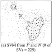
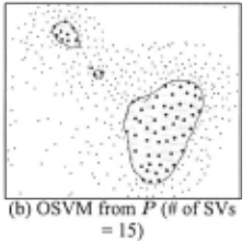
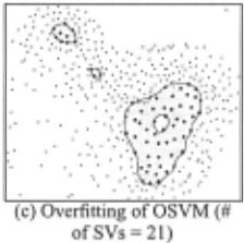
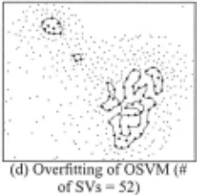
However, OSVM requires a much larger amount of positive training data to induce an accurate class boundary because its support vectors (SVs) of the boundary only comes from the positive data set and thus the small number of positive SVs can hardly cover the major directions of the boundary espe cially in high dimensional spaces. Due to the SVs coming only from positive data, OSVM tends to overfit and underfit easily. Tax proposed a sophisticated method which uses artif ically generated unlabeled data to optimize the OSVM's pa rameters that "balance" between overfitting and underfitting [Tax and Duin, 2001]. However, their optimization method is infeasibly inefficient in high dimensional spaces, and even with the best parameter setting, its performance still lags far behind the original SVM with negative data due to the short age ofSVs which makes "incomplete" the boundary descrip tion. Figure 1(a) and (b) show the boundaries of SVM and OSVM on a synthetic data set in a two-dimensional space. (We used LIBSVM version 2.33 1 for SVM implementation.) In this low-dimensional space with "enough" data, the ob stensibly "smooth" boundary ofOSVM is not the result of the good generalization but instead is from the poor expressibility caused by the "incomplete" SVs, which will become much worse in high-dimensional spaces where more SVs around the boundary are needed to cover major directions in the high dimensional spaces. When we increase the number ofSVs in OSVM, it overfits rather than being more accurate as shown in Figure 1(c) and (d).
1.2 Contributions and Paper Layout
We first discuss the "optimal" SCC boundary, which moti vates our new SCC framework Mapping-Convergence (MC), where the algorithms under the MC framework generate the boundary close to the optimum (Section 2). In Section 3, we present an efficient SCC algorithm Support Vector Mapping Convergence (SVMC) under the MC framework. We prove that although SVMC iterates under the MC framework for the "near-optimal" result, its training time is independent of the number of iterations, which is asymptotically equal to that of a SVM. We empirically verify our analysis of SVMC by extensive experiments on various domains of real data sets such as text classification (e.g., Web page classification), pat tern recognition (e.g., letter recognition), and bioinformatics (e.g., diagnosis of breast cancer), which shows the outstand ing performance of SVMC in a wide spectrum of SCC problems (with nominal or continuous attributes, linear or nonlin ear separation, and low or high dimensions) (Section 4).
1 http:/ /www.csie.ntu.edu. tw/ ""cj lin/libsvm
1.3 Notation
We use the following notation throughout this paper.
- xis a data instance such that x E U.
- P is a subspace for positive class within U, from which positive data set P is sampled.
- U (unlabeled data set) is a uniform sample of the univer sal set.
- U is the feature space for the universal set such that U ~ ~m where m is the number of dimensions.
For an example of Web page classification, the universal set is the entire Web, U is a uniform sample of the Web, P is a collection of Web pages of interest, and x E ~m is an instance of a Web page.
2 Mapping Convergence (MC) Framework
2.1 Motivation
In machine learning theory, the "optimal" class boundary function (or hypothesis) h(x) given a limited number of train ing data set { (x, l)} (l is the label of x) is considered the one that gives the best generalization performance which de notes the performance on "unseen" examples rather than on the training data. The performance on the training data is not regarded as a good evaluation measure for a hypothesis be cause the hypothesis ends up overfitting when it tries to fit the training data too hard. (When a problem is easy (to classify) and the boundary function is complicated more than it needs to be, the boundary is likely overfitted. When a problem is hard and the classifier is not powerful enough, the boundary becomes underfit.) SVM is an excellent example of super vised learning that tries to maximize the generalization by maximizing the margin and also supports nonlinear separa tion using advanced kernels, by which SVM tries to avoid overfitting and underfitting [Burges, 1998].
The "optimal" SCC classifier without labeled negative data also needs to maximize the generalization somehow with highly expressive power to avoid overfitting and underfitting. To illustrate an example of the "near-optimal" SCC bound ary without labeled negative data, consider the synthetic data set (Figure 2) simulating a real situation where within U, (1) the universal set is composed of multiple groups of data, (2)
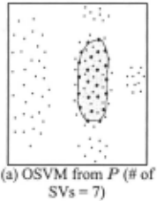
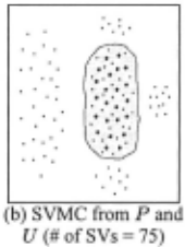
the positive class P is one of them (supposing P is the data group in the center), and (3) the positive data set P is a sam ple from P (assuming that the big dots are the sample P). OSVM draws P, a tight boundary around P, as shown in Figure 2(a), which overfits the true class area P due to the absence of the knowledge of the distribution of U. However, the "near-optimal" sec classifiers must locate the boundary between P and U outside P (Figure 2(b)) and thus maximize the generalization. The MC framework using U systemati cally draws the boundary of Figure 2(b ).
2.2 Negative Strength
Let h(x) be the boundary function of the positive class in U, which outputs the distance from the boundary to the instance x in U such that
h(x) > 0
h(x) < 0
lh(x)l > lh(x')l if xis a positive instance, if xis a negative instance, if xis located farther than x-'
from the boundary in U.
Definition 1 (Strength of negative instances). For two neg ative instances x and x' such that h(x) < 0 and h(x') < 0, ifih(x)l > lh(x')l. then xis stronger than x'.
Example 1. Consider a resume page classification function h(x) from the Web (U). Suppose there are two negative data objects x and x' (non-resume pages) in U such that h(x) < 0 and h(x') < 0: x is "how to write a resume" page, and x' is "how to write an article" page. In U, x' is considered more distant from the boundary of the resume class because x has more relevant features to the resume class (e.g., the word "resume" in text) though it is not a true resume page.
2.3 MC Framework
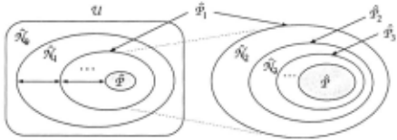
The MC framework is composed of two stages: the mapping stage and the convergence stage. In the mapping stage, the algorithm uses a weak classifier 1Ji1, which draws an initial approximation of "strong negatives" - the negative data lo cated far from the boundary of the positive class in U (steps 1 and 2 in Figure 4). Based on the initial approximation, the convergence stage runs in iteration using a second base classi fier 1Ji2, which maximizes the margin to make a progressively better approximation of negative data (steps 3 through 5 in Figure 4). Thus the class boundary eventually converges to the boundary around the positive data set in the feature space which also maximizes the margin.
Input:
-positive data set P , unlabeled data set U
Output:
- a boundary function h;
'lt 1: an algorithm identifying "strong negatives" from U
'lt2: a supervised learning algorithm that maximizes the margin
Algorithm:
- Use 'lt 1 to construct a classifier ho from P and U which classifies only "strong negatives" as negative and the others as positive
- Classify U by ho
- No := examples from U classified as negative by ho
- P0 := examples from U classified as positive by h0
3. Set N := 0 and i := 0
4. Do loop
4.1. N := N U fir;
4.2. Use 'lt2 to construct hH1 from P and N
- . Classify P; by hH1
- firH1 :=examples from P; classified as negative by hH1
- PH1 := examples from P; classified as positive by hH1 4.4. i := i + 1
4.5. Repeat until N; = 0
5. return h;
Figure 4: MC framework
Assume that P is a subspace tightly subsuming P within U where the class of the boundary function for P is from the algorithm 1Ji2 (e.g., SVM). In Figure 4, letN0 be the negative space and Po be the positive space within U divided by h0 (a boundary drawn by IJil), and let M be the negative space and Pi be the positive space within Pi- 1 divided by hi (a boundary drawn by 1Ji2). Then, we can induce the follow ing formulae from the MC framework of Figure 4. (Figure 3 illustrates an example of the spaces of the framework in U.)
where I is the number of iterations in the MC framework.
Theorem 1 (Boundary Convergence). Suppose U is uni formly distributed in U. If algorithm l]i 1 does not generate false negatives, and algorithm \}12 maximizes margin, then (1) the class boundary of the MC framework converges into the boundary that maximally separates P and U outside P, and (2) I (the number of iterations) is logarithmic in the margin between No and P.
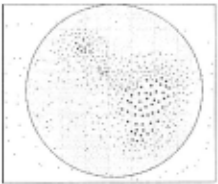
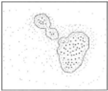
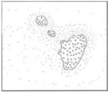
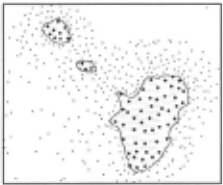
Figure 5: Intermediate results ofSVMC
Proof No n P = 0 because a classifier ho constructed by the algorithm \}1 1 does not generate false negative. A classifier h1 constructed by the algorithm \}12, trained from the separated space No and P, divides the rest of the space (U- (No+ P) which is equal to u{= 1 Nk) into two classes with a boundary that maximizes the margin between No and P. The first part becomes N1 and the other becomes u{=2Nk. Repeatedly, a classifier h;+l constructed by the same algorithm \}12, trained from the separated space U~=oNk and P, divides the rest of I~. ~ I ~· the space uk=i+1Nk mto N;+l and uk=i+2Nk Wlth equal margins. Thus, Ni+1 always has the margin of half of M (fori 2: 1). Therefore, I will be logarithmic in the margin between No and P.
The iteration stops when N; = 0, where there exists no sample of U outside P. Therefore, the final boundary will be located between P and U outside P while maximizing the margin between them. 0
Theorem 1 proves that under certain conditions, the final boundary will be located between P and U outside P. How ever, in the example of Figure 2(b ), our framework generates the "better" boundary located between P and U outside P because in theorem 1, we made a somewhat strong assump tion, i.e., U is uniformly distributed, to guarantee the bound ary convergence. In a more realistic situation where there is some distance 8 between classes-Figure 2 shows some gaps between classes-if the margin between hi+1 and N; becomes smaller than 8 at some iteration, the convergence stops be cause Ni+1 becomes empty. The margin between hi+1 and N; reduces by half at each iteration as the boundary hi+1 ap proaches to P and thus the boundary is not likely to stop con verging when it is far from P unless U is severely sparse. Thus, we have the following claim:
Claim 1. The boundary of MC is located between P and U outside P ifU and P are not severely sparse and there exists visible gaps between P and U.
Validity of the component algorithms 111 1 and ll12
1. \}1 1 must not generate false negatives.
Most classification methods have a threshold to control the trade-off between precision and recall. We can adjust the threshold of \}1 1 so that it makes near 100% recall by sacrific ing precision. (Some violations of this can be handled by the soft constraint of\}12 (e.g., SVM).) Determining the threshold can be intuitive or automatic when not concerning the pre cision quality much. The precision quality of \}11 does not affect the accuracy of the final boundary as far as it approxi mates a certain amount of negative data because the boundary will converge eventually. Figure 5 visualizes the boundary af ter each iteration of SVMC. The mapping stage only identi fies very strong negatives by covering a wide area around the positive data (Figure 5(a)). (We used OSVM for the algorithm \}1 1 of the mapping stage. We intuitively set the parameters of OSVM such that it covers all the positive data without much concern for false positives.) Although the precision quality of mapping is poor, the boundary at each iteration converges (Figures 5(b) and (c)), and the final boundary is very close to the true boundary drawn by SVM with P and N (Figure l(a) and 5(d)). Our experiments in Section 4 also show that the final boundary becomes very accurate although the initial boundary of the mapping stage is very rough by the "loose" setting of the threshold of \}1 1.
2. \}1 2 must maximize margin.
SVM and Boosting are currently the most popular supervised learning algorithms that maximize the margin. With a strong mathematical foundation, SVM automatically finds the opti mal boundary without a validation process and without many parameters to tune. The small numbers of theoretically moti vated parameters also work well for an intuitive setting. For these reasons, we use SVM for \}12 for our research. In prac tice, the soft constraint of SVM is necessary to cope with noise or outliers. The soft constraint of SVM can affect I and the accuracy of the final boundary. However, P is not likely to have a lot of noise in practice because it is usually carefully collected by users. In our experiments, a low setting (i.e., v = 0.01) ofv (the parameter to control the rate of noise in the training data) performs well for all cases for this reason. (We used v-SVM for the semantically meaningful parameter [Chang and Lin, 2001].)
3 Support Vector Mapping Convergence (SVMC)
3.1 Motivation
The classification time of the final boundary of SMC ("Sim ple" MC with IJ12 = SV M) is equal to that of SVM because the final boundary is a boundary function of'IJ12 · The training time ofSMC can be very long if lUI is very large because the training time of SVM highly depends on the size of data set n (~ lUI), and SMC runs iteratively. tsMc = O(IUI2 *logiUI) assuming the number of iterations ~log lUI and tsv M = O(IUI2) where tw is the training time of a classifier IJT . (tsv M is known to be at least quadratic to n and linear to the number of dimensions). Refer to [Chang and Lin, 2001] for more discussion on the complexity of SVM. However, de creasing the sampling density of U to reduce the training time hurts the accuracy of the final boundary because the density of U will directly affect the quality of the SVs of the final boundary.
3.2 SVMC
SVMC prevents the training time from increasing dramat ically as the sample size grows. We prove that although SVMC iterates under the MC framework for the "near optimal" result, its training time is independent of the number of iterations, and thus its training time is asymptotically equal to that of a SVM.
The approach of SVMC is to use minimally required data set at each iteration such that the data set does not degrade the accuracy of the boundary while it saves the training time of each SVM maximally. To illustrate how SVMC achieves this, consider the point of starting the third iteration (when i == 2) in SMC. (See step 4.1 in Figure 4.) After we merge N2 into N, we may not need all the data from N in order to construct h3 because the data far from h3 may not contribute to the SVs. The set of negative SVs of h2 is the representative data set for No and N1, so we only keep the negative SVs of h2 and the newly induced data set N2 to support the negative side of h3.
Claim 2 (Minimally required negative data). Minimally required negative data at ( i + 1 )th iteration (Vi ~ 1) that makes h;+l is as accurate as the boundary constructed from UJ=oNi and P, is N; U negative support vectors of h;.
Rationale. The negative SVs of hi+1 will be from k and the negative SV s of h; because N; is the closest data set to h;+l and because the directions not supported by N; in the feature space will be supported by the negative SVs of h;, which are the representing data set for u~:;,~Ni. However, if any of the negative SVs of h; is excluded in constructing h;+l , h;+l might suffer because the negative SV s of h; need to support the direction that N; does not support in the feature space. Thus, N; U negative support vectors of h; are the minimally required negative data set at (i + 1)th iteration.
D
For the minimally required data set for the positive side, we cannot definitely exclude any data object from P at each iteration because positive SVs are determined depending on negative SVs, and it is hard to determine the positive data that cannot be SVs independent of negative SVs or SVM parame ters.
Surprisingly, adding the following statement between step 4.4 and 4.5 of the original MC framework of Figure 4 com pletes the SVMC algorithm.
Reset N with negative SVs of IJ12
Theorem 2 (Training time of SVMC). Suppose tsv M O(n 2 ), and INi+ll = ll}l, Vi~ 1. Then, tsvMc = O(n 2 ).
Proof For simplicity of the proof, we approximate each value as follows.
D
Theorem 2 states that the training complexity of SVMC is asymptotically equal to that of SVM. Our experiments in Section 4 also show that SVMC trains much faster than SMC while it remains the same accuracy. Figure 5 visualizes the boundary after each iteration of SVMC on the same data set ofFigure 1.
4 Empirical Results
In this section, we show the empirical verification of our anal ysis on SVMC by extensive experiments on various domains of real data sets - Web page classification, letter recognition, and diagnosis of breast cancer - which show the outstand ing performance of SVMC in a wide spectrum of SCC prob lems (with nominal or continuous attributes, linear or nonlin ear separation, and low or high dimensions).
4.1 Datasets and Methodology
Due to space limitations, we reports only the main results. Our evaluation is based on the F1 measure (F1 = 2pr j (p + r), pis precision and r is recall) as was used in [Liu eta!., 2002] - one of the most recent works on sec from positive and unlabeled data 2 · We also report the accuracy.
We used the letter recognition and breast cancer data sets from the UCI machine learning repository 3 for direct com parisons with OSVM. (OSVM is often used for letter or digit recognition [Tax and Duin, 2001].) We also used Webkb 4 for Web page classification as used in [Liu eta!., 2002] for the indirect comparison with it. We set up the experiment en vironment in the same way as [Liu eta!., 2002], except our setup is more realistic: In [Liu et al., 2002], U is composed of b% of positives (e.g., student) and samples from another class (e.g., course). Our U is b% of positives (e.g., student) and the remainder is from all other classes. (Refer to [Liu et al., 2002] for the rest of the data set description.)
2 Refer to [Liu eta/., 2002] for the justification of using the Fl measure for sec.
3 http://www. ics.uci .edu/~mlearn!MLRepository.htrnl
| Class | IPI | lUI | IPul | Fl, Accuracy(%) | T-Time (sec.) | |||||
|---|---|---|---|---|---|---|---|---|---|---|
| TSVM | SMC | SVMC | usVM | SVM_NN | SMC | SVMC | ||||
| letter 'A' | 521 | 10007 | 384 | 0.9929, 99.96 | 0.9840, 99.91 | 0.9840, 99.91 | 0.8457, 99.22 | 0.0811' 97.26 | 171.77 | 45.37 |
| 'B' | 521 | 10004 | 377 | 0.9651 , 99.83 | 0.9046, 99.50 | 0.9204, 99.59 | 0.7207, 98.69 | 0.0834, 97.58 | 75.61 | 14.34 |
| 'C' | 485 | 9996 | 371 | 0.9860, 99.23 | 0.9641, 99.82 | 0.9641, 99.82 | 0.7354, 98.82 | 0.0758, 97.55 | 155.70 | 29.93 |
| 'D' | 525 | 10050 | 402 | 0.9820, 99.91 | 0.9300, 99.63 | 0.9300, 99.63 | 0.6921,98.60 | 0.0902, 97.52 | 80.47 | 16.06 |
| 'E' | 518 | 10026 | 392 | 0.9798, 99.90 | 0.9419, 99.70 | 0.9396, 99.69 | 0.7112, 98.78 | 0.1333, 97.64 | 98.13 | 21.57 |
| b-cancer | 135 | 259 | 77 | 0.9628, 98.87 | 0.9585, 98.75 | 0.9585, 98.75 | 0.6315, 83.32 | 0.2434, 36.06 | 0.131 | 0.025 |
| course | 482 | 4179 | 448 | 0.8969, 97.82 | 0.8259, 96.65 | 0.8434, 96.89 | 0.2028, 36.59 | 0.0880, 89.30 | 636.70 | 143.29 |
| faculty | 532 | 4209 | 592 | 0.9032, 97.68 | 0.8420, 95.89 | 0.8705, 96.58 | 0.2621 , 50.11 | 0.0168, 86.05 | 749.63 | 217.85 |
| student | 816 | 4154 | 825 | 0.9240, 97.27 | 0.8495, 94.29 | 0.8505, 94.15 | 0.3384, 32.52 | 0.0000,80.14 | 1181.59 | 296.50 |
4.2 Results
Table 4 shows the performance results. TSVM (Traditional SVM) shows the ideal performance using SVM from P and manually classified N from U. SVM_NN (SVM with Noisy Negatives) is SVM from P, with U as a substitute for N . (U can be thought of as a good approximation of N.) Note that for TSVM, SVM_NN, and MC (SMC and SVMC), we used theoretically motivated fixed parameters without performing explicit optimization or validation process. For OSVM, we thoroughly searched for the best parameters based on the test ing data set since optimizing parameters as specified in [Tax and Duin, 2001] is infeasibly inefficient especially in high di mensional spaces.
MC (SMC and SVMC) without labeled negative data show performance close to that of TSVM. SVMC trains much faster than SMC for most data sets. The performance ofSMC and SVMC is comparable. (They differ a little because of the soft constraints of SVM and noise in the data.) OSVM per forms fairly well on letter recognition and breast cancer (of low dimensionality with large amounts of data) but poor on Webkb (of high dimensionality). SVM_NN suffers from very low Fl scores because negative prediction dominates due to many false positives in the training data.
5 Conclusion
We present the MC framework and its instance algorithm SVMC, a new SCC method from positive and unlabeled data (without labeled negative data). SVMC without labeled nega tive data computes an accurate classification boundary around the positive data using the distribution of unlabeled data in a systematic way.
4 http: //www-2.cs.cmu.edu/afs/cs.cmu.edu/project/theo lllwww/wwkb/
@inproceedings{ijcai2003p84,
  title     = {SVMC: Single-Class Classification With Support Vector Machines},
  author    = {Yu, Hwanjo},
  booktitle = {Proceedings of the Eighteenth International Joint Conference on
               Artificial Intelligence, {IJCAI-03}},
  publisher = {International Joint Conferences on Artificial Intelligence},
  editor    = {Georg Gottlob and Toby Walsh},
  pages     = {567--573},
  year      = {2003},
  url       = {https://ijcai.org/proceedings/2003/84},
}
TY - CPAPER TI - SVMC: Single-Class Classification With Support Vector Machines AU - Yu, Hwanjo T2 - Proceedings of the Eighteenth International Joint Conference on Artificial Intelligence, IJCAI-03 PB - International Joint Conferences on Artificial Intelligence PY - 2003 SP - 567 EP - 573 UR - https://ijcai.org/proceedings/2003/84 ER -Copied
Machine-readable versions of this paper, for tools and AI agents:





