
Generalized Target Assignment and Path Finding Using Answer Set Programming
Proceedings of the Twenty-Sixth International Joint Conference on Artificial Intelligence. Main track. Pages 1216-1223.
https://doi.org/10.24963/ijcai.2017/169
Keywords
- Knowledge Representation, Reasoning, and Logic: Action, Change and Causality
- Planning and Scheduling: Applications of Planning
Abstract
In Multi-Agent Path Finding (MAPF), a team of agents needs to find collision-free paths from their starting locations to their respective targets. Combined Target Assignment and Path Finding (TAPF) extends MAPF by including the problem of assigning targets to agents as a precursor to the MAPF problem. A limitation of both models is their assumption that the number of agents and targets are equal, which is invalid in some applications such as autonomous warehouse systems. We address this limitation by generalizing TAPF to allow for (1)~unequal number of agents and tasks; (2)~tasks to have deadlines by which they must be completed; (3)~ordering of groups of tasks to be completed; and (4)~tasks that are composed of a sequence of checkpoints that must be visited in a specific order. Further, we model the problem using answer set programming (ASP) to show that customizing the desired variant of the problem is simple one only needs to choose the appropriate combination of ASP rules to enforce it. We also demonstrate experimentally that if problem specific information can be incorporated into the ASP encoding then ASP based method can be efficient and can scale up to solve practical applications.
- [Boyarski et al., 2015] Eli Boyarski, Ariel Felner, Roni Stern, Guni Sharon, David Tolpin, Oded Betzalel, and Solomon Shimony. ICBS: Improved conflict-based search algorithm for multi-agent pathfinding. In Proceedings of the International Joint Conference on Artificial Intel- ligence, pages 740-746, 2015. IJCAI
- [Cohen et al., 2016] Liron Cohen, Tansel Uras, T. K. Satish Kumar, Hong Xu, Nora Ayanian, and Sven Koenig. Im- proved solvers for bounded-suboptimal multi-agent path finding. In Proceedings of the International Joint Confer- ence on Artificial Intelligence, pages 3067-3074, 2016. IJCAI
- [de Wilde et al., 2014] Boris de Wilde, Adriaan ter Mors, and Cees Witteveen. Push and Rotate: A complete multi- agent pathfinding algorithm. Journal of Artificial Intelli- gence Research, 51:443-492, 2014.
- [Erdem et al., 2013] Esra Erdem, Doga Kisa, Umut Öztok, and Peter Schüller. A general formal framework for pathfinding problems with multiple agents. In Proceedings of the AAAI Conference on Artificial Intelligence, pages 290-296, 2013.
- [Gebser et al., 2014] Martin Gebser, Roland Kaminski, Ben- jamin Kaufmann, and Torsten Schaub. Clingo = ASP + control: Preliminary report. CoRR, abs/1405.3694, 2014.
- [Gelfond and Lifschitz, 1988] M. Gelfond and V. Lifschitz. The stable model semantics for logic programming. In Proceedings of the International Conference on Logic Pro- gramming, pages 1070-1080, 1988.
- [Goldenberg et al., 2014] Meir Goldenberg, Ariel Felner, Roni Stern, Guni Sharon, Nathan Sturtevant, Robert Holte, and Jonathan Schaeffer. Enhanced Partial Expansion A*. Journal of Artificial Intelligence Research, 50:141-187, 2014.
- [Lifschitz and Turner, 1994] V. Lifschitz and H. Turner. Splitting a logic program. In Pascal Van Hentenryck, edi- tor, Proceedings of the International Conference on Logic Programming, pages 23-38, 1994.
- [Lifschitz, 2002] V. Lifschitz. Answer set programming and plan generation. Artificial Intelligence, 138(1-2):39-54, 2002.
- [Luna and Bekris, 2011] Ryan Luna and Kostas Bekris. Push and Swap: Fast cooperative path-finding with complete- ness guarantees. In Proceedings of the International Joint Conference on Artificial Intelligence, pages 294- 300, 2011. IJCAI
- [Ma and Koenig, 2016] Hang Ma and Sven Koenig. Optimal target assignment and path finding for teams of agents. In Proceedings of the International Conference on Au- tonomous Agents and Multiagent Systems, pages 1144- 1152, 2016.
- [Morris et al., 2016] Robert Morris, Corina Pasareanu, Kasper Luckow, Waqar Malik, Hang Ma, T. K. Satish Kumar, and Sven Koenig. Planning, scheduling and monitoring for airport surface operations. In Proceedings of Planning for Hybrid Systems Workshop, 2016.
- [Sharon et al., 2015] Guni Sharon, Roni Stern, Ariel Felner, and Nathan Sturtevant. Conflict-based search for optimal multi-agent pathfinding. Artificial Intelligence, 219:40- 66, 2015.
- [Silver, 2005] David Silver. Cooperative pathfinding. In Proceedings of the AAAI Conference on Artificial Intelli- gence and Interactive Digital Entertainment, pages 117- 122, 2005.
- [Simons et al., 2002] P. Simons, N. Niemelä, and T. Soini- nen. Extending and implementing the stable model se- mantics. Artificial Intelligence, 138(1-2):181-234, 2002.
- [Surynek et al., 2016a] Pavel Surynek, Ariel Felner, Roni Stern, and Eli Boyarski. Efficient SAT approach to multi- agent path finding under the sum of costs objective. In Proceedings of the European Conference on Artificial In- telligence, pages 810-818, 2016.
- [Surynek et al., 2016b] Pavel Surynek, Ariel Felner, Roni Stern, and Eli Boyarski. An empirical comparison of the hardness of multi-agent path finding under the makespan and the sum of costs objectives. In Proceedings of the Sym- posium on Combinatorial Search, pages 145-147, 2016.
- [Veloso et al., 2015] Manuela Veloso, Joydeep Biswas, Brian Coltin, and Stephanie Rosenthal. CoBots: Robust symbiotic autonomous mobile service robots. In Proceed- ings of the International Joint Conference on Artificial Intelligence, pages 4423-4429, 2015. IJCAI
- [Wagner and Choset, 2015] Glenn Wagner and Howie Choset. Subdimensional expansion for multirobot path planning. Artificial Intelligence, 219:1-24, 2015.
- [Wang and Botea, 2011] Ko-Hsin Cindy Wang and Adi Botea. MAPP: A scalable multi-agent path planning algo- rithm with tractability and completeness guarantees. Jour- nal of Artificial Intelligence Research, 42:55-90, 2011.
- [Wurman et al., 2008] Peter Wurman, Raffaello D'Andrea, and Mick Mountz. Coordinating hundreds of coopera- tive, autonomous vehicles in warehouses. AI Magazine, 29(1):9-20, 2008.
- [Yu and LaValle, 2016] Jingjin Yu and Steven LaValle. Op- timal multirobot path planning on graphs: Complete al- gorithms and effective heuristics. IEEE Transaction on Robotics, 32(5):1163-1177, 2016.
References were extracted automatically from the PDF and may contain errors.
Full text extracted automatically from the PDF; figures, tables and equations may differ. The PDF is the version of record.
1 Introduction Categories and Subject Descriptors
In MAPF, the objective is to find collision-free paths for agents moving to their goal locations while minimizing either the makespan or the total path cost. Researchers have proposed various optimal and boundedly-suboptimal algorithms [Goldenberg et al., 2014; Wagner and Choset, 2015; heuristic search; Kiva (Amazon Robotics) systems; multiagent path finding; multi-robot path finding; network flow; path planning; robotics; target assignment; team work; warehouse automation Appears in: Proceedings of the 15th International Conference on Autonomous Agents and Multiagent Systems (AAMAS 2016), J. Thangarajah, K. Tuyls, C. Jonker, S. Marsella (eds.), May 9-13, 2016, Singapore.
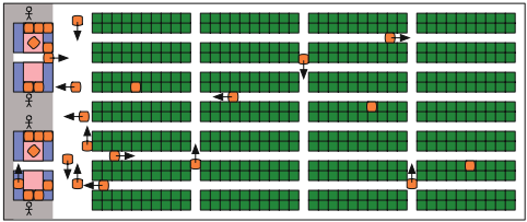
Multi-Agent Path Finding (MAPF) deals with teams of agents that need to find collision-free paths from their respective starting locations to their respective goal locations on a graph. This model can be applied to a number of applications including autonomous aircraft towing vehicles [Morris et al., 2016], autonomous warehouse systems [Wurman et al., 2008], office robots [Veloso et al., 2015], and video games [Silver, 2005]. For example, in an autonomous warehouse system (illustrated by Figure 1), robots (in orange) navigate around a warehouse to pick up inventory pods from their storage locations (in green) and drop them off at designated inventory stations (in purple) in the warehouse. We use this as our motivating application throughout this paper. I.2.8 [Artificial Intelligence]: Problem Solving, Control Methods, and Search-graph and tree search strategies, heuristic methods; I.2.11 [Artificial Intelligence]: Distributed Artificial Intelligence-intelligent agents, multiagent systems General Terms Algorithms, Performance, Experimentation Keywords
1. INTRODUCTION
used to move the inventory pods with the correct bins from
anonymous MAPF (multi-agent path-finding) problems:
Figure 2: A Kiva drive unit and storage pod. their storage locations to the inventory stations where a pick worker removes the desired products from the desired bin. Note that the pod has four faces, and the drive unit may need to rotate the pod in order to present the correct face. When a picker is done with a pod, the drive unit stores it in an empty storage location. Each station is equipped with a desktop computer that controls pick lights, barcode scanners, and laser pointers that are used to identify the pick and put locations. Because every product is scanned in and out of the system, overall picking errors go down, which potentially eliminates the need for post-picking quality control. In general, every station is capable of being either a picking station or a replenishment station. In practice, pick stations will be located near outbound conveyors, and replenishment stations will be located near pallet drop off points. The power of the Kiva solution comes from the fact that it allows every worker to have random access to any inventory in the warehouse. Moreover, inventory can be retrieved in parallel. When the picker is filling several boxes at the same time, the parallel, random access ensures that she is not waiting on pods to arrive. In fact, by keeping a small queue of work at the station, the Kiva system delivers a new pod face every six seconds, which sets a baseline picking rate of 600 lines per hour. 2 Peak rates can exceed 600 lines per hour when the operator can pick more than one item off a pod. 3 For a large warehouse, the savings in personnel can be significant. Consider, for example, what a Kiva implementation of the book warehouse would involve. A busy bookseller may ship 100,000 boxes a day. With existing automation, this level of output would employ perhaps 75 workers 2 This statistic is based on single unit picks and has been reproduced for extended periods in the Kiva test facility. 3 This statistic was verified when a small Kiva demonstration system was brought to a drugstore distribution center where operators picked at nearly 700 lines per hour. 1755 Teams of agents often have to assign targets among themselves and then plan collision-free paths to their targets. Examples include autonomous aircraft towing vehicles [12], automated warehouse systems [22], office robots [19] and game characters in video games [15]. For example, in the near future, autonomous aircraft towing vehicles might tow aircraft all the way from the runways to their gates (and vice versa), reducing pollution, energy consumption, congestion and human workload. Today, autonomous warehouse robots already move inventory pods all the way from their storage locations to the inventory stations that need the products they store (and vice versa), see Figure 1. We therefore study the TAPF (combined targetassignment and path-finding) problem for teams of agents in known terrain. The agents are partitioned into teams. Each team is given the same number of unique targets (goal locations) as there are agents in the team. The TAPF problem is to assign agents to targets and plan collision-free paths for the agents from their current locations to their targets in a way such that each agent moves to exactly one target given to its team, all targets are visited and the makespan (the earliest time step when all agents have reached their targets and stop moving) is minimized. Any agent in a team can be assigned to a target of the team, and the agents in the same team are thus exchangeable. However, agents in di↵erent teams are not exchangeable. 1.1 RelatedWork The TAPF problem generalizes the anonymous and nonSharon et al., 2015; Boyarski et al., 2015; Cohen et al., 2016] as well as suboptimal ones [Wang and Botea, 2011; Luna and Bekris, 2011; de Wilde et al., 2014]. While most of them are search-based, there are also approaches that reformulate the problem using answer set programming [Erdem et al., 2013], mixed-integer programming [Yu and LaValle, 2016], and satisfiability testing [Surynek et al., 2016a]. Ma and Koenig [2016] recently generalized MAPF to combined Target Assignment and Path Finding (TAPF), where agents are partitioned into teams and each team is given a set of targets that they need to get to. To solve this problem, one must first find an assignment of targets to agents before solving the resulting MAPF problem. While TAPF better reflects real-world systems with homogeneous agents, such as our motivating application, it still has a key limitation: It assumes that the number of agents equals the number of tasks to be allocated. In our motivating application, there are typically more tasks than agents. As such, agents have to move towards a new task after completing their current task. Therefore, we propose Generalized TAPF (G-TAPF), a generalization of TAPF that allows the number of tasks to be greater than the number of agents. We also propose a new objective, which better captures more applications including our motivating warehouse application: Each task has an associated deadline that indicates the time at which it must be completed. We propose to use answer set programming (ASP) [Lifschitz, 2002] as the general framework for solving the new G-TAPF problems. Empirical results show that it is
Copyright c©2016, International Foundation for Autonomous Agents and Multiagent Systems (www.ifaamas.org). All rights reserved.
- The anonymous MAPF problem (sometimes called goal-invariant MAPF problem) results from the TAPF problem if only one team exists (that consists of all
more scalable than existing TAPF algorithms, using imperative programming, for some TAPF problem types.
The rest of the paper is organized as follows. We begin with a brief review of ASP and multi-shot ASP. We then present a precise definition of G-TAPF problems. Afterwards, we describe our ASP encoding of G-TAPF problems. Afterwards, we describe two algorithms for computing solutions of GTAPF problems that use the ASP-encoding of G-TAPF, one for computing optimal solution and another for non-optimal solution. Next, we evaluate the performance of our algorithms using two sets of TAPF problems and a set of G-TAPF problems.
2 Background: ASP andMulti-shot ASP
A logic program Π is a set of rules of the form
where 0≤m≤n, each ai is an atom of a propositional language and not represents (default) negation. An atom is of form p(c1, ..., ck), where p is a k-ary predicate, also written as p/k, and each cj is a constant. Intuitively, a rule states that if all positive literals ai are believed to be true and no negative literal not ai is believed to be true, then a0 must be true. If a0 is omitted, the rule is called a constraint. If n = 0, it is called a fact. For a rule r as in (1), head(r) denotes a0; pos(r) (positive body) denotes the set {a1, . . . , am}; and neg(r) (negative body) denotes {am+1, . . . , an}. Also, we let lit(r) denote the set of all literals in r, viz. {head(r)}∪pos(r)∪{not a | a ∈ neg(r)}; accordingly, lit(P) denotes the set of all literals of logic program Π. Semantically, a program induces a collection of so-called answer sets, which are distinguished models determined by answer sets semantics; see [Gelfond and Lifschitz, 1988] for details.
To facilitate the use of ASP in practice, several extensions have been developed. First of all, rules with variables are viewed as shorthands for the set of their ground instances. Further language constructs include conditional literals and cardinality constraints [Simons et al., 2002]. The former are of form a : b1, . . . , bm, the latter can be written as s{d1, . . . , dn}t, where a and bi are possibly default negated literals, and each dj is a conditional literal; s and t provide optional lower and upper bounds on the number of satisfied literals within the cardinality constraints. We refer to b1, . . . , bm as a condition. The practical value of both constructs becomes more apparent when used in conjunction with variables. In ASP, strings starting with uppercase (lowercase) letter are typically used to denote variables (constants). For instance, a conditional literal of form a(X) : b(X) in a rule's antecedent expands to the conjunction of all instances of a(X) for which the corresponding instance of b(X) holds. Similarly, 2{a(X) : b(X)}4 is true, whenever more than one and less than five instances of a(X) (subject to b(X)) are true. Aggregate functions such as count, sum, etc. are also introduced. For example, count {X : a(X)} computes the number of different objects X such that condition a(X) is true. Finally, a simply yet useful construct is that of a range, that is, a fact p(1..n) stands for the set of facts p(1) to p(n).
Traditional ASP solvers are single-shot solvers, i.e., they take a logic program, compute its answer sets, and exit.
Recently developed multi-shot ASP solvers provide operative solving processes for dealing with continuously changing logic programs. For controlling such solving processes, the declarative approach of ASP is combined with imperative means. In clingo [Gebser et al., 2014], this is done by augmenting an ASP encoding with Python procedures controlling ASP solving processes along with the corresponding evolving logic programs. The instrumentation includes methods for adding/grounding rules, setting truth values of atoms, 1 computing the answer sets of current program, etc.
3 Generalized TAPF Problems
A Generalized TAPF (G-TAPF) problem is given by a triple P = (G, R, T ), where
- G = (V,E) is an undirected connected graph, where V and E correspond to locations and ways of moving between locations for the agents;
- R is a set of agents. Each r ∈ R is specified by a pair (t, s), t is the type of task that can be accomplished by r and s ∈ V is the starting location of r;
- T is a set of groups of tasks. Each group in T is specified by a set of orders O and a positive integer d representing the deadline of the orders in the group; each o ∈ O is a pair (g, t) where g and t are the destination and type of the order, respectively.
For an agent r, type(r) and loc(r) denote the type and starting location of agent r, respectively. For a task t, type(t) and destination(t) denote the type and destination of task t, respectively. For a group T of tasks, deadline(T) denotes the deadline of tasks in group T .
Agents can move between the vertices along the edges of G, one edge at a time, under the restrictions: (a) two agents cannot swap locations in a single timestep; and (b) each location can be occupied by at most one agent at any time. A path for an agent r is a sequence of vertices α = 〈v1, . . . , vn〉 if (i) the agent starts at v1 (i.e., v1 = loc(r)); and (ii) if for any two subsequent vertices vi and vi+1, there is an edge between them (i.e., (vi, vi+1) ∈ E) or they are the same vertex (i.e., vi = vi+1). n is called the length of α and is denoted by length(α).
An agent r completes a task t via a path α = 〈v1, . . . , vn〉 if type(r) = type(t) and destination(t) is one of the vertices in α, i.e., destination(t) ∈ {v1, . . . , vn} . A task is said to be completed when an agent completes it. A group of tasks is completed when every task in the group is completed. A G-TAPF problem P is completed when every group of tasks in T is completed. A solution of a G-TAPF problem P is a collection of paths S = {αr | r ∈ R} for the agents in R so that all tasks in T are completed.
Depending on the application, one can create different GTAPF variants. We describe several variants below:
- Equal numbers of tasks and agents: This variant is the original TAPF [Ma and Koenig, 2016], where there is a one-toone allocation of tasks to agents.
1 The manipulation of truth values is restricted to atoms explicitly declared as being external.
- Group completion: Agents must complete all groups of tasks in some order. More precisely, for every pair of distinct groups of tasks, all tasks in one group must be completed before all tasks in the other group.
- Task deadlines: Agents must complete all the tasks t ∈ Ti within a group Ti within the deadline of the group deadline(Ti).
- Completion with checkpoints: In order to complete a task t, before and/or after reaching the goal destination(t), an agent must visit some other designated checkpoints. Under this view, the autonomous warehouse system [Wurman et al., 2008] can also be viewed as a G-TAPF variant, where to complete a task t, an agent needs to pick up a pod at a checkpoint before bringing it to the inventory station (= destination(t)) and then returning the pod to another checkpoint.
One can optimize different possible objectives:
- The makespan of a solution S is defined by maxα∈S length(α). Minimizing this value is appropriate if one wants to minimize the total time taken by the agents to complete all the tasks in the problem. Alternatively, one can also seek to find a solution whose makespan is within a maximum makespan threshold. which is appropriate in problems where there is a deadline in which to complete all the tasks.
- The total path cost of a solution S is defined by ∑α∈S length(α). Minimizing this value is appropriate if the cost of a path is measured by fuel consumption and one wants to minimize the total amount of fuel used. As above, one can also seek to find a solution whose total path cost is within a maximum threshold.
A discussion between the tradeoffs of the objectives for MAPF problems can be found in [Surynek et al., 2016b]. In this paper, we focus on minimizing the makespan.
4 Modeling G-TAPFs Using ASP
Let P =(G, R, T ) be a G-TAPF problem and n be an integer denoting the upper bound on the solution makespan.
4.1 G-TAPF Input Representation
We represent edges and vertices in a graph G by e(x, y) and v(r) atoms, respectively. Agents are specified by ag(a, l, t) atoms (a: agent identifier, l: starting location, t: type). Groups of tasks are specified by grp(g, d) atoms (g: group identifier, d: deadline for the tasks in g). Tasks are specified by task(i, g, l, t) atoms (i: task identifier, g: group identifier of i, l: destination, t: type).
4.2 G-TAPF ASP Rules
We assume a set of atoms of the form st(0), . . . , st(n), each st(i) represents a timestep in a solution of P. We use atoms of the form at(r, l, s) with the intuitive meaning "agent r is at location l at timestep s."
Action Generation
We use atoms of the form mv(r, l, s) (respectively, stay(r, l, s)) to denote that agent r moves to (respectively, stays at) the vertex l in timestep s. At any timestep S, an agent R at location L executes exactly one action of either moving to a connected location L′ (mv(R, L′ , S)) or staying at L (stay(R, L, S)). The next rule generates an action for an agent R at timestep S with this restriction:
The starting location of an agent is specified by:
The next two rules allow for reasoning about the locations of the agents. The first rule encodes the effect of the action mv and the second rule encodes the effect of the action stay.
The next two rules enforce the constraints on the movements of the agents. Rule (6) prevents two agents from moving to the same location at the same timestep and Rule (7) prevents two agents to exchange locations in a single timestep.
Task Allocation
Rule (8) assigns tasks to agents. It ensures that each task t is assigned to exactly one agent r of the correct type (i.e., type(t) = type(r)) and defines the atom goal(r, t, l, o) whenever agent r is assigned task t whose destination is at location l and whose ordering is o and is encoded by atoms of the form order(g, o) (defined in the next group).
Group Completion
When group completion needs to be enforced, one needs to create an ordering for the groups of tasks to be completed. The set of rules in this group defines atoms of the form order (g, o) which says that the group of tasks g must be completed at the oth order among all groups. It assumes that a Boolean flag ordering indicating the necessity of group completion has been specified. We start by counting the number of the groups:
Next, each group is assigned an order using the rules (10) and (11). Rule (10) assigns the order of each group to a number between 1 and the number of groups. Rule (11) assigns 1 as the order of each group if the ordering flag is false which is equivalent to saying that there is no order between the groups.
To ensure that no two groups have the same order if the ordering flag is true, we include the following constraint:
Solution Verification, Checkpoints, Deadlines
Rules for solution verification need to check for the achievement of tasks as well as the satisfaction of various requirements such as group completion, deadlines, and checkpoints. When the problem requires multiple checkpoints, the Boolean flag checkpoint is set to true and each task t is associated with a sequence [l1, . . . , lx] where li ∈ V and the goal of t, g, occurs in [l1, . . . , lx]; the checkpoints are defined (explicitly or implicitly) using atoms of the form chkp(t, li, i).
As an example, consider the autonomous warehouse system problem. Assume that each task t with goal g has three checkpoints: The agent must first go to a storage location store(g, s) to pick up the pod, then to an inventory location (goal g), before going back to a possibly different storage location depot(g, s) to store the pod. Then, the specification of the checkpoints for this problem can be specified by the following rules:
Having defined and specified the checkpoints of the problems, we now introduce the set of rules to check for the completion of the individual tasks.
(16) defines that the destination of a task is the first checkpoint for a task if checkpoint is false. (17) counts the number of checkpoints for each task.
Rules (18)-(22) define the predicate com/4, where com(r, t, k, s) means that agent r has visited the kth checkpoint of the task t at timestep s. They ensure that only a visit to the (k +1)th checkpoint after visiting the kth checkpoint is counted towards a solution. Rule (18)-(19) define this atom for tasks in the 1st group (ordering 1) and rules (20)-(21) for tasks in the oth , o > 1, group. Observe that rules (20)- (21) are applicable only if finished(o - 1, s) is true, which is defined in (23)-(24). When a checkpoint has been visited at timestep s - 1, it means that it has been visited at timestep s. This is encoded in rule (22).
The next two rules define finished(o, s) indicating that the group of tasks with ordering o is completed at s. Rule (23) computes the number of tasks in a group and Rule (24) states that finished(o, s) is true whenever all tasks in the group are completed.
Finally, the next constraint ensures that every agent completes all the targets assigned to it:
To take into account deadlines, a Boolean flag deadline is set to true if deadlines need to be enforced. In addition to checking for task completion, deadlines of tasks need to be verified. This is achieved by the following constraint:
The constraint says that if agent r is assigned task t with goal g and deadline d, then at timestep d, the task must be completed. Note that because of (22), the constraint requires that the task is completed on or before the deadline. Furthermore, because of (25), the task must be completed on or before timestep n. As such, this constraint does not need to be considered for groups with deadlines beyond n.
It is worth pointing out that the constraint (26) assumes that the last checkpoint of the task must be visited on or before the deadline. In some situations, this assumption might be not necessary, i.e., a task could be considered as completed at the time the agent visits some other checkpoints such as the task's destination (e.g., in the autonomous warehouse application, delivering the goods at the station could be used to indicate that the task has been completed even though the robot will still need to a depot). The constraint can be easily modified to take into consideration other settings.
5 Solving G-TAPFs
We first describe how to find a solution with makespan n, assuming it exists, before describing how to find a solution with the minimal makespan. Using built-in optimization features of ASP solvers, one can generalize our methods for other objectives (e.g., minimizing the total path cost).
5.1 SolutionWithMakespan n
Let Π(P, n, o, d, c) be the program consisting of the input and Rules (2)-(26), where o, d, and c denote the ordering, deadline, and checkpoint flags, respectively. Let A be an answer set of Π(P, n, o, d, c). It is easy to see that for each agent r, A must contain some atom of the form at(r, vs, s) for each timestep s = 0, . . . , n due to Rules (3)-(5). So, we define αr(A) = 〈v0, . . . , vn〉 where at(r, vj , j) ∈ A for j = 0, . . . , n.
Proposition 1 Let P=(G,R, T) be a G-TAPF program, n an integer, and Q=Π(P, n, o, d, c). It holds that
- for each answer set A of Q,
- S = {αr(A) | r ∈ R} is a solution of P; - If o is true then for every pair of groups g1 and g2 in T, either all the tasks in g1 are completed before all the tasks in g2 or vice versa.
- If d is true then, for every groups g with the deadline d, all tasks in g are completed before timestep d + 1. - For every task t completed by an agent r, there is a proper ordering of the checkpoints of t in αr(A).
- Q is consistent iff P has a solution with makespan at most n and every solution of with makespan at most n of P can be computed by Q.
- Q is inconsistent iff P does not have a solution with makespan at most n.
Proof. (Sketch)
- Proof for the first property:
- Since A is an answer set of Π(P, n, o, d, c), rule (25) must be satisfied. Consider an atom goal(r, i, g, o) in A. Rule (25) implies that com(r, i, g, n) belongs to A, which implies that there exists some s ≤ n such that at(r, g, s) ∈ A (by the rules (18)-(22)). By the construction of αr(A), we have r completes the task i of group with the order o. By the rule (8), we have that each task of the problem is assigned to one robot. Since all robots will complete their assigned tasks, we have that S is a solution of P .
- If o is true, then rules (9)-(12) imply that each group of tasks is assigned a number o between 1 and |T| (the number of groups in T ), i.e., for each group g there exists a unique order(g, o) ∈ A. Rules (18)-(22) ensure that if order(g1, o1) and order(g2, o2) belong to A then all tasks in g1 are completed before all tasks in g2 which proves the property.
- If d is true, then by definition o is also true. The above item, together with the rule (26), ensures that tasks in the group with earlier deadline will be completed before tasks in the group with the later deadline.
- Proof of the second property followed from the first property and the fact that given a solution S, one can construct an answer set AS such that αr(AS) = S.
- The third property follows from the first and second property. □
5.2 SolutionWith The Minimal Makespan
The first method for finding a solution with the minimal makespan utilizes the program Π(P, n, o, d, c) by searching for the smallest n∗ such that Π(P, n∗ , o, d, c) has an answer set and Π(P, n∗ - 1, o, d, c) does not. It implements Algorithm 1 in multi-shot ASP and consists of the program Π(P, n, o, d, c) and a Python program inc GTAPF(P) which is responsible for instantiating Π(P, i, o, d, c) with the input P and i, computing an answer set of Π(P, i, o, d, c), and extracting solutions. In Algorithm 1, Gi and Πi denote the set of ground instantiations of Rules (25)-(26) and the ground program obtained from Π(P, n, o, d, c) without (25)-(26) for n = i, respectively.
Proposition 2 For a G-TAPF problem P, (i) if inc GTAPF(P) returns (〈αr〉r∈R, i), then 〈αr〉r∈R is an optimal solution of P with makespan i; (ii) if inc GTAPF(P) returns (timeout, i), then P does not have a solution with makespan at most i - 1.
Algorithm 1: inc GTAPF(P) Input: G-TAPF problem P = (G, R, T ). Output: a solution, its makespan i; or timeout. 1 i = 1; Π = Π1 ∪G1 2 while not(timeout) do 3 if Π has an answer set then 4 compute an answer set Z of Π 5 extract 〈αr〉r∈R fromZ, i.e., αr = αr(Z) 6 return (〈αr〉r∈R, i) 7 Π = (Π \Gi) ∪ (Πi+1 \ Πi) ∪Gi+1; i = i +1 8 return (timeout, i) Algorithm 2: d GTAPF(P) Input: G-TAPF problem P = (G, R, T ). Output: a solution, its makespan i; or timeout. 1 Compute an answer set AG of ΠG(P) 2 nT = {o | order( , o) ∈ AG} 3 i = 0 4 Π = Πi ∪AG 5 while nT ̸= ∅ and not(timeout) do 6 k = min{o | o ∈ nT} 7 Π = Π∪ (Πi+1 \ Πi) ∪Gki+1 8 i = i +1 9 while not(timeout) do 10 if Π has an answer set then 11 compute an answer set Z of Π 12 extract 〈αr〉r∈R fromZ, i.e., αr = αr(Z) 13 add action occurrences in Z to Π 14 break 15 Π = (Π \ Gki ) ∪ (Πi+1 \ Πi) ∪ Gki+1 16 i = i +1 17 nT = nT \ {k} 18 Π = Π \Gki 19 if not(timeout) then return (〈αr〉r∈R, i) 20 return (timeout, i)5.3 Greedy Strategy
The previous subsection presents a straightforward method that uses the general ASP encoding of a G-TAPF problem for computing its optimal solution. This can be inefficient as the length of the optimal solution increases. The culprit lies in Lines 3-6 of inc GTAPF(P), which requires a call to the answer set solver, and the fact that if Π(P, i, o, d, c) has no answer set, an answer set solver needs to consider all feasible orderings of the groups of tasks when group completion (c is true) is required. One way to address this issue is to greedily assign an ordering among the tasks when c is true. We next present an algorithm that implements this idea. First, we begin with a short discussion of the theoretical foundation that guarantees the correctness of the algorithm.
Let ΠG(P) be the program consisting of the input and (8)-(12). Furthermore, ΠS(P, n, o, d, c) = Π(P, n, o, d, c) \ ΠG(P). Intuitively, ΠG(P) is the program that generates the goal assignment for the robots. This assignment must satisfy the requirements of P (e.g., ordering of groups when group completion is required). It is easy to see that lit(ΠG(P)), the set of literals occurring in ΠG(P), is a splitting set of Π(P, n, o, d, c). Due to the Splitting Theorem in [Lifschitz and Turner, 1994], A is an answer set of Π(P, n, o, d, c) iff A = AG ∪AS, where AG is an answer set of ΠG(P ) and AS is an answer set of Π′S (P, n, o, d, c), which is obtained from Π(P, n, o, d, c) by (i) deleting every rule r ∈ Π(P, n, o, d, c) such that (pos(r)∩lit(ΠG(P)))\AG ̸= ∅ or neg(r)∩AG ̸= ∅; and (ii) replacing every remaining rule r by a rule r′ where head(r′ ) = head(r), pos(r′ ) = pos(r) \ lit(ΠG(P)), and neg(r′ ) = neg(r)\lit (ΠG(P )). Furthermore, it can be shown that A is also an answer set of Π(P, n, o, d, c) ∪ AG.
The above discussion suggests that an answer set A=AG∪AS of Π(P, n, o, d, c) can be computed by computing an answer set (i) AG of ΠG(P); and (ii) A of Π(P, n, o, d, c) ∪ AG. This strategy is implemented in Algorithm 2 with an additional refinement that focuses on the ordering of the groups; e.g., we focus on completing tasks in the first order before working on the second order. Goi to denote the set of ground instantiations of Rules (25)-(26) for all atoms of the form goal (r, i, g, o) ∈ AG.
Algorithm 2 computes an answer set AG of ΠG(P) (Line 1) that contains atoms of the form order(g, o) which specifies the ordering between the groups of tasks (the set nT). It then computes solutions for the groups according to this ordering (Lines 5-18). When Π(P, i, o, d, c) has an answer set, the set of action occurrences are extracted and added to the program (Line 13) to maintain that the tasks that are completed stay completed when searching for the solution of the next group of tasks. Similar to Proposition 2, we can prove the soundness of Algorithm 2.
Proposition 3 For a G-TAPF problem P, if d GTAPF(P) returns (〈αr〉r∈R, i), then 〈αr〉r∈R is a solution of P with makespan i.
6 Experimental Evaluation
We perform experimental evaluations on three benchmarks with different G-TAPF variants, including the TAPF formulation. In TAPF problems, we compare our ASP approach against CBM, the only TAPF algorithm proposed thus far [Ma and Koenig, 2016]. We conducted our experiments on a 3.60GHz CPU machine with 8GB of RAM, and set a timeout of 1800s.
6.1 Gridworld
We vary the grid size, and the number of agents, groups, and tasks. Blocked cells, agent starting locations, and task locations are randomly selected. We report the percentage of instances solved (out of 10) within the time limit, and both the average runtimes (in seconds) and makespans of the instances solved.
Table 1 tabulates the results. CBM is able to solve TAPF problems at least one order of magnitude faster than our ASPbased algorithm. In general, the runtimes of the ASP-based algorithm increase as the makespans of solutions found increase. Finally, the ASP-based algorithm is faster on problems with deadlines and without ordering constraints than on problems with ordering constraints and no deadlines. The reason is that the program needs to enforce more rules when ordering constraints are necessary than when deadlines are necessary.
| Grid | No. of | No. of | No. of Tasks | ASP | CBM | Make- | ||
|---|---|---|---|---|---|---|---|---|
| Size | Agents | Groups | Comp | Time | Comp | Time | span | |
| 10x10 | 50 40 50 50 30 | 1 1 10 5 4 | 80 80 50 50 40 | 100% 100% 100% 100% 100% | 6.0 2.8 9.2 249.2 13.3 | 100% 100% | 0.045 0.025 | 2.0 2.0 8.9 6.7 5.7 |
| 20x20 | 20 15 20 5 | 1 1 2 2 | 20 30 20 10 | 90% 100% 100% 90% | 1.3 6.6 12.8 100.4 | 100% 100% | 0.024 0.064 | 8.0 8.9 12.7 13.6 |
| 10x10 | 50 40 50 50 30 | 1 1 10 5 4 | 80 80 50 50 40 | 100% 100% 100% 100% 100% | 6.1 2.9 420.9 60.3 62.1 | 2.0 2.0 13.0 8.0 | ||
| 7.6 | ||||||||
| 20 | 1 | 20 | 100% | 2.4 | 100% | 0.024 | 8.4 | |
| 20x20 15 | 1 | 30 | 100% | 6.1 | 9.0 | |||
| 20 | 2 | 20 | 100% | 14.5 | 12.8 | |||
| 5 | 2 | 10 | 40% | 39.9 | 11.8 |
| 10x10 | 50 40 50 50 | 1 1 10 5 | 80 80 50 20 | 100% 100% 100% 100% | 6.0 2.8 8.2 3.6 | 2.1 2.0 8.9 6.7 |
| 100% | 1.3 | 5.7 | ||||
| 30 | 4 | 40 | ||||
| 20 | 1 | 20 | 100% | 53.1 | 8.4 | |
| 20x20 15 | 1 | 30 | 100% | 6.3 | 9.0 | |
| 20 | 2 | 20 | 100% | 12.9 | 12.8 | |
| 5 | 2 | 10 | 90% | 102.9 | 13.2 |
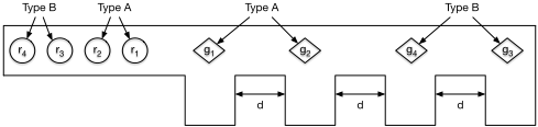
Figure 2: Example CORRIDOR Layout
6.2 Corridor
A limitation of gridworlds is that it does not allow us to parameterize the difficulty of the problem in terms of the number of conflicts if each agent takes its shortest path to its goal. In fact, in many of the instances, the number of such conflicts is quite small, favoring CBM. We thus propose a new benchmark, called CORRIDOR, for TAPF problems. Figure 2 illustrates an example instance. In this benchmark, there is a long corridor, whose width is exactly one cell except for goal cells, which have a width of two cells. We parameterize the size of the state space via the distance d between two goal cells and the number of conflicts via the ordering of groups of goals. There are no conflicts when the groups of goals and agents have the same ordering (from left to right) and maximum conflicts when their orderings are reversed (e.g., in Figure 2).
Table 2 tabulates the results for TAPF problems with 20 agents/tasks in 10 groups. When the number of conflicts is small (≤ 25 for d = 1 and ≤ 20 for d = 2), CBM is faster than our ASP algorithm. However, as the number of conflicts increases, CBM slows down substantially and times out for the more difficult problems. On the other hand, the runtime of our ASP algorithm increases more slowly, allowing it to also solve the more difficult problems. This result shows that our ASP approach may be more suitable in more complex (G-)TAPF problems.
| No. of Conflicts | d = 1 | ||||||
|---|---|---|---|---|---|---|---|
| ASP Time | CBM Time | Make- span | ASP Time | d = 2 CBM Time | Make- span | ||
| 0 | 6.378 | 0.142 | 40 | 15.899 | 0.211 | 60 | |
| 5 | 7.067 | 0.177 | 42 | 17.186 | 0.366 | 62 | |
| 10 | 8.021 | 0.123 | 44 | 18.375 | 0.403 | 64 | |
| 15 | 8.021 | 0.123 | 44 | 18.391 | 0.427 | 64 | |
| 20 | 8.594 | 0.365 | 46 | 19.823 | 0.631 | 66 | |
| 25 | 9.523 | 0.675 | 48 | 21.265 | 247.544 | 68 | |
| 30 | 9.647 | 54.81 | 48 | 21.431 | 274.525 | 68 | |
| 35 | 10.714 | timeout | 50 | 22.849 | 67.665 | 70 | |
| 40 | 12.754 | timeout | 54 | 26.341 | timeout | 74 | |
| 45 | 12.932 | timeout | 54 | 31.112 | timeout | 78 | |
| Config. | Original Map Size | No. of Agents | No. of Groups | No. of Tasks | Simplified Map Size | ASP W Runtime | Makespan |
|---|---|---|---|---|---|---|---|
| 2×2×10 | 186*354 | 4 | 2 | 4 | 107*286 | 6 | 296 [6] |
| 3×3×10 | 350*734 | 8 | 4 | 3 | 227*470 | 18 | 731 [9] |
| 3×4×10 | 460*960 | 8 | 4 | 3 | 301*624 | 55 | 1004 [10] |
| 4×4×10 | 598*1250 | 10 | 4 | 5 | 398*826 | 87 | 1076 [10] |
| 5×4×10 | 741*1544 | 10 | 1 | 10 | 496*1030 | 276 | 483 [16] |
| 5×4×10 | 741*1544 | 10 | 2 | 10 | 496*1030 | 392 | 776 [13] |
| 5×4×10 | 741*1544 | 20 | 1 | 15 | 496*1030 | 803 | 535 [17] |
| 6×4×10 | 874*1830 | 10 | 1 | 10 | 594*1278 | 431 | 604 [14] |
| 6×4×10 | 874*1830 | 10 | 2 | 10 | 594*1278 | 876 | 1095 [14] |
| 6×4×10 | 874*1830 | 20 | 1 | 15 | 594*1278 | 1501 | 778 [16] |
| 7×4×10 | 1012*2120 | 10 | 2 | 10 | 689*1432 | 1300 | 1232 [16] |
| 7×4×10 | 874*1830 | 20 | 1 | 15 | 689*1432 | timeout | - |
6.3 Autonomous Warehouse System
As G-TAPFs are motivated by applications such as autonomous warehouse systems, we included this domain as well. We use various warehouse configurations similar to the one in Figure 1. In these problems, each task has three checkpoints - the initial storage location, the inventory station, and the final storage location. Each configuration is denoted by r ×c×p, where r, c, and p are the number of rows, columns, and inventory pods per block, respectively. The example in Figure 1 thus has a 7 × 4 × 10 configuration. Problems in this domain prove to be extremely hard for the ASP encoding presented earlier. In fact, it cannot solve the 2 × 2 × 10 configuration because the size of the graph contains 168 nodes and 354 edges, and the length of the optimal solutions is often over 30 steps due to the presence of multiple checkpoints. For this reason, we developed an enhancement of the proposed method to tackle these problems. We call this encoding warehouse encoding and denote it with ASP W. The source code and a demo of this experiment is available at https://potassco.org/labs/.
ASP W relies on the observation that the paths for agents can be found using the following steps: (i) simplifying the original map to a simpler map with fewer nodes and edges; (ii) computing the simplified paths for agents using the simplified map; and (iii) computing the actual solution using the simplified paths on the original map. These steps are feasible due to the fact that several nodes in a warehouse do not have full connectivity (e.g., an inventory pod might be connected to a single node). This allows for nodes whose connectivity degree is less than or equal 3 to be grouped together into a combined node. This reduces the size of the graph and the length of the solutions (in the reduced graph) to the extent that it becomes manageable for the greedy encoding. Further, we divide each task into three subtasks, one for each checkpoint. This simplification is reasonable as the number of tasks in a group is usually no larger than the number of available agents to perform those tasks.
Table 3 tabulates the results, where we vary the r × c × p configuration and the number of agents, groups of tasks, and tasks per group. For each configuration, we generate three instances, average the results, and report the size (|nodes| ∗ |edges|) of the simplified map, the average ASP W runtime, and the average makespan of the solution. We also report the average path length to complete a subtask in the simplified map in boldface between brackets. It can be seen that (i) this average path length for a subtask is a good indicator for the difficulty of the problem for ASP W; and (ii) smaller configurations with more agents and tasks are more difficult than larger configurations with fewer agents and tasks (e.g., configuration 5×4×10 with 20 agents and 1 group of 15 tasks is harder to solve than configuration 6 × 4 × 10 with 10 agents and 1 group of 10 tasks).
7 Conclusions
Both MAPF and TAPF models suffer from their limiting assumption that the number of agents and targets are equal. In this paper, we propose the Generalized TAPF (G-TAPF) formulation that allows for (1) unequal number of agents and tasks; (2) tasks to have deadlines by which they must be completed; (3) ordering of groups of tasks to be completed; and (4) tasks that are composed of a sequence of checkpoints that must be visited in a specific order. As different G-TAPF variants may be applicable in different domains, we model them using ASP, which allows one to easily customize the desired variant by choosing appropriate combinations of rules to enforce. Our experimental results show that CBM is better in simple TAPF problems with few conflicts, but worse in difficult problems with more conflicts. We also show that ASP technologies can easily exploit domain-specific information to improve its scalability and efficiency. The contributions in this paper thus make a notable jump towards deploying MAPF and TAPF algorithms in practical applications.
Acknowledgements
We thank Hang Ma and Sven Koenig for sharing with us their implementation of the CBM solver for TAPF problems. We would also like to thank all the reviewers for their constructive comments and suggestions. Finally, this research is partially support by DFG (550/9) and NSF grant 1345232. The views and conclusions contained in this document are those of the authors and should not be interpreted as representing the official policies, either expressed or implied, of the sponsoring organizations, agencies, or the U.S. government
@inproceedings{ijcai2017p169,
  title     = {Generalized Target Assignment and Path Finding Using Answer Set Programming},
  author    = {Nguyen, Van and Obermeier, Philipp and Son, Tran Cao and Schaub, Torsten and Yeoh, William},
  booktitle = {Proceedings of the Twenty-Sixth International Joint Conference on
               Artificial Intelligence, {IJCAI-17}},
  publisher = {International Joint Conferences on Artificial Intelligence Organization},
  editor    = {Carles Sierra},
  pages     = {1216--1223},
  year      = {2017},
  month     = {8},
  note      = {Main track},
  doi       = {10.24963/ijcai.2017/169},
  url       = {https://doi.org/10.24963/ijcai.2017/169},
}
TY - CPAPER TI - Generalized Target Assignment and Path Finding Using Answer Set Programming AU - Nguyen, Van AU - Obermeier, Philipp AU - Son, Tran Cao AU - Schaub, Torsten AU - Yeoh, William T2 - Proceedings of the Twenty-Sixth International Joint Conference on Artificial Intelligence, IJCAI-17 PB - International Joint Conferences on Artificial Intelligence Organization PY - 2017 SP - 1216 EP - 1223 DO - 10.24963/ijcai.2017/169 UR - https://doi.org/10.24963/ijcai.2017/169 ER -Copied
Machine-readable versions of this paper, for tools and AI agents:





