
Causality Based Propagation History Ranking in Social Networks
Proceedings of the Twenty-Fifth International Joint Conference on Artificial Intelligence. Pages 3917-3922.
© 2016 International Joint Conferences on Artificial Intelligence
Abstract
In social network sites (SNS), propagation histories which record the information diffusion process can be used to explain to users what happened in their networks. However, these histories easily grow in size and complexity, limiting their intuitive understanding by users. To reduce this information overload, in this paper, we present the problem of propagation history ranking. The goal is to rank participant edges/nodes by their contribution to the diffusion. Firstly, we discuss and adapt Difference of Causal Effects (DCE) as the ranking criterion. Then, to avoid the complex calculation of DCE, we propose a resp-cap ranking strategy by adopting two indicators. The first is responsibility which captures the necessary face of causal effects. We further give an approximate algorithm for this indicator. The second is capability which is defined to capture the sufficient face of causal effects. Finally, promising experimental results are presented to verify the feasibility of our method.
- [Campbell et al., 1997] John Y Campbell, Andrew Wen- Chuan Lo, Archie Craig MacKinlay, et al. The economet- rics of financial markets, volume 2. princeton University press Princeton, NJ, 1997.
- [Chen et al., 2015] Shuo Chen, Ju Fan, Guoliang Li, Jianhua Feng, Kian-lee Tan, and Jinhui Tang. Online topic-aware influence maximization. Proceedings of the VLDB Endow- ment, 8(6):666-677, 2015.
- [Chockler and Halpern, 2004] Hana Chockler and Joseph Y Halpern. Responsibility and blame: A structural-model approach. Journal of Artificial Intelligence Research, 22:93-115, 2004. IJCAI
- [Chvatal, 1979] Vasek Chvatal. A greedy heuristic for the set-covering problem. Mathematics of operations re- search, 4(3):233-235, 1979.
- [Eiter and Lukasiewicz, 2002] Thomas Eiter and Thomas Lukasiewicz. Complexity results for structure-based causality. Artificial Intelligence, 142(1):53-89, 2002. IJCAI
- [Fisher, 1925] Ronald Aylmer Fisher. Statistical methods for research workers. Genesis Publishing Pvt Ltd, 1925.
- [Freire et al., 2015] Cibele Freire, Wolfgang Gatterbauer, Neil Immerman, and Alexandra Meliou. The complex- ity of resilience and responsibility for self-join-free con- junctive queries. Proceedings of the VLDB Endowment, 9(3):180-191, 2015.
- [Guille et al., 2013] Adrien Guille, Hakim Hacid, Cécile Favre, and Djamel A Zighed. Information diffusion in on- line social networks: A survey. ACM SIGMOD Record, 42(2):17-28, 2013.
- [Hume, 1739] David Hume. A treatise of human nature. London: John Noon, 1739.
- [Kitsak et al., 2010] Maksim Kitsak, Lazaros K Gallos, Shlomo Havlin, Fredrik Liljeros, Lev Muchnik, H Eu- gene Stanley, and Hernán A Makse. Identification of in- fluential spreaders in complex networks. Nature Physics, 6(11):888-893, 2010.
- [Kleinberg and Hripcsak, 2011] Samantha Kleinberg and George Hripcsak. A review of causal inference for biomedical informatics. Journal of biomedical informat- ics, 44(6):1102-1112, 2011.
- [Kleinberg, 2003] Jon Kleinberg. Bursty and hierarchical structure in streams. Data Mining and Knowledge Dis- covery, 7(4):373-397, 2003.
- [Lewis, 1973] David Lewis. Causation. The Journal of Phi- losophy, 70(17):556-567, 1973.
- [Li et al., 2015] Jiuyong Li, Lin Liu, and Thuc Le. Practical Approaches to Causal Relationship Exploration. Springer, 2015.
- [McAuley and Leskovec, 2012] Julian J McAuley and Jure Leskovec. Learning to discover social circles in ego net- works. In Neural Information Processing Systems (NIPS), volume 272, pages 548-556, 2012.
- [Meliou et al., 2010a] Alexandra Meliou, Wolfgang Gatter- bauer, Joseph Y Halpern, Christoph Koch, Katherine F Moore, and Dan Suciu. Causality in databases. IEEE Data Eng. Bull., 33(3):59-67, 2010.
- [Meliou et al., 2010b] Alexandra Meliou, Wolfgang Gatter- bauer, Katherine F Moore, and Dan Suciu. The complexity of causality and responsibility for query answers and non- answers. Proceedings of the VLDB Endowment, 4(1):34- 45, 2010.
- [Milgram, 1967] Stanley Milgram. The small world prob- lem. Psychology today, 2(1):60-67, 1967.
- Lavon B Page and Jo Ellen Perry. Reliability polynomials and link importance in networks. IEEE Transactions on Reliability, 43(1):51-58, 1994.
- [Pearl, 2000] Judea Pearl. Causality: models, reasoning and inference. Cambridge Univ Press, 2000.
- [Qin et al., 2013] Biao Qin, Shan Wang, Xiaofang Zhou, and Xiaoyong Du. Responsibility analysis for lineages of con- junctive queries with inequalities. IEEE Transactions on Knowledge and Data Engineering, 2013.
- [Salganik and Heckathorn, 2004] Matthew J Salganik and Douglas D Heckathorn. Sampling and estimation in hid- den populations using respondent-driven sampling. Socio- logical methodology, 34(1):193-240, 2004.
- [Strang and Aarikka, 1986] Gilbert Strang and Kaija Aarikka. Introduction to applied mathematics, volume 16. Wellesley-Cambridge Press Wellesley, MA, 1986.
- [Wasserstein, 1997] Ronald L Wasserstein. Monte carlo: Concepts, algorithms, and applications. Technometrics, 39(3):338-338, 1997.
References were extracted automatically from the PDF and may contain errors.
Full text extracted automatically from the PDF; figures, tables and equations may differ. The PDF is the version of record.
1 Introduction
Online social networks have been requisite for modern life. Every day, massive amounts of posts (tweets, messages) are emerging and disseminating in social network sites (SNS). Usually, a user may receive the same news from several different followees or friends. At this time, the user might want to know why (s)he could receive this post, or what is each involved user's role in the propagation. Luckily, propagation histories, which record the diffusion process, are partially provided to users in some online SNS, such as Sina Weibo (the Chinese counterpart of Twitter).
Example 1 (Propagation history of a diffusion on Weibo). Bill Gates posts a message about his speech on Weibo, and Tom receives this news via Delx (one of his followees). This repost trace is recorded and illustrated on Tom's homepage. In addition, the other two propagation traces are included, i.e., via Alice/Cain and Alice/Bob respectively. This propagation history (top in Fig. 1) could explain why Tom could receive this news or who plays the key role in this diffusion.
⇤Corresponding author: Chaokun Wang.
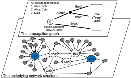
Note that only propagation histories, rather than the underlying network topology, are used to explain information diffusion in this study. An illustration of Example 1 is given in Fig. 1. We can see that these recorded propagation traces exactly capture users' repost behaviors in the dynamic flow of information regardless of the underlying network topology. With these traces, we can intuitively explain this diffusion, e.g., Alice tends to be an important person since there are two propagation traces going through this user.
However, propagation histories can rapidly grow in size and complexity, making it difficult to understand intuitively. To reduce this information overload, in this paper, we present the problem of propagation history ranking. The goal is to rank propagation participants (edges/nodes) by their contribution to the diffusion. As such, we put forward our solution from the viewpoint of causality [Hume, 1739]. Causality based reasoning has long been a hot topic in cognitive science research areas, and could draw a clear picture of each participant's contribution during the propagation.
More Applications. Another interesting application is network reliability [Page and Perry, 1994]: Given a network, identify the important edges/nodes to guarantee its connectivity. However, in practice, the entire network structure is not always available, e.g., for security reasons. The distribution records of gateways, a kind of propagation history, might be considered to prioritize the diagnosis work.
Contributions. Our contributions are as follows:
- To the best of our knowledge, we are the first to study the propagation history ranking problem in SNS. We further discuss and adapt Difference of Causal Effects (DCE) as the ranking criterion.
- We propose a "resp-cap" ranking strategy (to avoid the hardness of DCE calculation) by adopting indicators responsibility and capability to capture the necessary and sufficient faces of causal effects, respectively.
- We give an approximate algorithm for responsibility calculation, since this problem is generally NP-hard.
- Extensive experiments on real-world datasets demonstrate the feasibility of our ranking mechanism.
2 Preliminary and Problem Statement
In this paper, we restrict our discussion to the information diffusion from one source node to one target node. Without loss of generality, we consider edges as propagation participants. Following this, we give a formal definition of propagation history and its ranking problem.
Definition 1 (Propagation history of a diffusion). The propagation history of a diffusion in SNS records all the actual propagation trails of an event E from the source S to the target T , and is usually formalized as:
where each ti is called a trace, constructed by li ordered edges (ti1 ↪ ▷▷▷↪ tili ). We drop the subscript (E↪S↪T ) when there is no ambiguity.
Propagation history ranking. Let Φ be the propagation history of a diffusion, and let T be the edge set of Φ. The goal is to rank those edges in T by their contribution to this diffusion.
3 DCE as Ranking Criterion
In this section, we discuss how to estimate the edge importance in propagation histories, and introduce the selected ranking criterion.
Importance Estimation. The concernwith regard to the importance of a specific edge concentrates on two effects: What is the overall effect on this diffusion if this edge fails? Or what is the effect if the edge is non-failed? Considering the likelihood of a successful transmission, these two effects can be estimated as:
- ÷ P(Φx0=true) is the probability of a successful information transmission if edge X is intervened to be failed.
- ÷ P(Φx=true) is the probability of a successful information transmission if edge X is intervened to be nonfailed.
Note that, x and x0 stand for interventions to set edge X to be "non-failed" and "failed" in randomized experiments [Fisher, 1925], respectively. Therefore, P(Φx0=true)
and P(Φx=true) are two causal effect measures considering how necessary and sufficient the edge is for the diffusion, respectively. It is natural to consider the above two effects together, i.e., the Difference of Causal Effects, (DCE) [Pearl, 2000]:
Consequently, DCE considers both necessary and sufficient faces of causal effects, and a rigorous proof can be found in [Pearl, 2000]. The similar idea is widely adopted in other research areas, such as network reliability [Page and Perry, 1994] and economics [Campbell et al., 1997].
DCE Calculation. To calculate this causal measure, adopting randomized experiments is the preferred golden method [Fisher, 1925]. We briefly describe this procedure as follows. Given the input edge X, we first enforce X to be "non-failed" (or "failed"). Then, in each simulation, we randomly set the other participant edges to be failed or nonfailed, and further check if the diffusion would be successful. After a great number of simulations, we get the probability of P(Φx=true) (or P(Φx0=true)). Finally, we would get the DCE value according to Eq. 1.
4 Integrated "resp-cap" Ranking Strategy
Although conducting randomized experiments is preferred for DCE calculation, this method needs to run simulations many times over to obtain a convergent value [Wasserstein, 1997]. To avoid this complication, we propose a "resp-cap" ranking strategy by adopting two indicators (i.e., responsibility and capability) to capture the intuition of causal effects from two faces.
4.1 Responsibility
To capture the necessary face of causal effects in a diffusion, we introduce the concept of responsibility [Chockler and Halpern, 2004] based on the following definition inspired by [Pearl, 2000].
Definition 2 (Causality in a diffusion). Suppose the edge set of the propagation history is T. Let t 2 T be a participant edge, and let Γ ⇢ T be an edge set. t is called a cause for this diffusion w.r.t. Γ, if the following two conditions are satisfied:
- The diffusion from s to t remains with T-Γ, and
- after removing Γ, the removal of t would make this diffusion fail.
Γ is called the contingency set for t.
Although checking causality (i.e., evaluating each cause and its related contingency set) is NP-complete in general [Eiter and Lukasiewicz, 2002], [Meliou et al., 2010b] gave a PTime solution for provenance data of relational databases. This method would be directly applied to the propagation history in SNS. In this paper, we only focus on the causality based ranking problem.
Definition 3 (Responsibility). Suppose the edge set of the propagation history is T , and let t 2 T be a participant edge. The responsibility of t for this diffusion is:
where Γ ranges over all contingency sets for t.
Example 2 (Example 1 continued). The propagation history of this diffusion is Φ=¶t1 ↪ t2 ↪ t3 ♦, where t1=(A↪B), t2=(A↪C) and t3=(D). The responsibility of edge A is 1/2, because the smallest contingency set for A is ¶D♦. Similarly, the responsibility of D is 1/2 with the smallest contingency set ¶A♦. The smallest contingency sets for B and C are ¶C, D♦ and ¶B, D♦, respectively. Therefore, their responsibility values are both 1/3.
Responsibility of edge t is determined by the minimum edge set whose removal will make t indispensable for a successful information transmission, which leads to the following proposition.
Proposition 1. Responsibility measures the necessary face of causal effects.
Proof. The proof is based on a causal measure Probability of Necessary (PN), which is defined as the probability of event y would not have occurred in the absence of event x, given that x and y did in fact occur [Pearl, 2000]. Therefore, PN measures the necessary face of causal effects.
Let X be a participant edge, and let x and x0 stand for the propositions "X non-failed" and "X failed" respectively. Let set S contain all propagation traces which go through edge X, and the rest of the traces are put into another set (denoted as ¯ S). Let s and ¯ s stand for the cases that S and ¯ S can successfully transmit the information respectively, and let s0 and ¯ s0 denote their complements. We could calculate the PN value of edge X: PN = P(¯ s0 s)◁[P (¯ sx) + P (¯ s0 s)]. Suppose every edge follows the same failure probability 50%. Then we get the following equations:
As the responsibility of X increases, ¯ S becomes easier to get broken (P(¯ s0 ) increases and P(¯ s) decreases). In this case, if P(s) keeps the same, PN will increase. Therefore, responsibility has a positive relationship with PN, i.e., responsibility measures the necessary face of causal effects.
Complexity of Responsibility. In theory, to compute the responsibility one has to iterate over all contingency sets, i.e., computing responsibility in general is NP-hard [Chockler and Halpern, 2004]. Therefore, we propose an approximate algorithm, and more details can be found in Section 5.
4.2 Capability
To capture the sufficient face of causal effects in a diffusion, we define the concept of capability.
Definition 4 (Capability). Suppose the edge set of the propagation history is T, and let t 2 T be a participant edge. The capability of t for this diffusion is:
where Ł ranges over all propagation traces going through t, and function st(Ł) returns the edge set of Ł.
Example 3 (Example 1 continued). The capability of edge A is 1/2, since it needs edge ¶B♦ or ¶C♦ to ensure the diffusion. The capability values of B and C are both 1/2, because both of them need ¶A♦ to get information transmitted. Edge D's capability is 1 because D itself can guarantee the diffusion.
The capability of edge t is determined by the minimum edge set whose addition could make t indispensable for a successful information transmission, which leads to the following proposition.
Proposition 2. Capability measures the sufficient face of causal effects.
Proof. The proof is based on a causal measure Probability of Sufficiency (PS). As stated in [Pearl, 2000], PS is defined as the probability of enabling x would produce y in a situation where x and y are in fact absent. Therefore, PS measures the sufficient face of causal effects.
Continuing with the same definitions of X, x, x0 , S, ¯ S, s, ¯ s, s0 and ¯ s0 in the proof of Proposition 1, we can calculate the PS value of edge X: PS = P (¯ s0 (s♣x)x0 )◁P (¯ s0x0 )▷ First of all, since ¯ S consists of the traces which do not contain edge X, P(¯ s) and P (¯ s0 ) are not affected by X. As ⇢x (the capability of X) increases, P(s♣x) increases, i.e., S becomes easier to ensure the diffusion. Since P(¯ s0 ) and P(x0 ) are not affected by ⇢x, PS will increase when ⇢x increases. Therefore, capability has a positive relationship with PS, i.e., capability measures the sufficient face of causal effects.
Complexity of Capability. Suppose the propagation history contains N traces and M edges. Using an inverted index, calculating the capability values of all edges can be done in O(LN) (with O(M) space complexity), where L is the average length of all propagation traces. Generally, L is not a large number according to the concept of six degrees of separation [Milgram, 1967]. Therefore, the capability problem has a linear complexity with respect to the number of propagation traces.
4.3 Integrated "resp-cap" Ranking
By combining the above two indicators, we get the integrated "responsibility-capability" ranking strategy (short for "respcap") defined as follows:
where fn stands for a normalized function calculating the standard score [Strang and Aarikka, 1986] and 0<↵<1 is a balance factor. Note that these two indicators can be incorporated into other more complex ranking methods, which we leave as our future work.
5 Approximate Algorithm for Responsibility
Since responsibility is hard to calculate, in this section, we propose an approximate algorithm which guarantees a feasible solution. We first compare the responsibility problem with the classical set cover problem (SCP) [Chvatal, 1979]. Responsibility vs. SCP. Suppose the propagation history is organized for SCP: Φ=¶c1↪ ▷ ▷ ▷ ↪ cn♦, where ci is a subset of the whole participant edge set T = ¶t1↪ ▷ ▷ ▷ ↪ tm♦. We assume function sc(tj↪Φ) = ¶ci♣tj2ci ^ ci2Φ♦ (sc(tj) for short), and intuitively sc(tj) covers (contains) all the sets (in Φ) containing tj. Given an edge t, the intuition of SCP is to find the minimum k which satisfies sc(t1) [ ▷ ▷ ▷ [ sc(tk) = Φ - sc(t). Responsibility problem has the same intuition, besides which it has another constraint that the removal of ¶t1↪ ▷ ▷ ▷ ↪ tk♦ must ensure t is still a cause for this diffusion, i.e., sc(t1) [ ▷ ▷ ▷ [ sc(tk) 6= Φ.
Approximate Algorithm for Responsibility. If Γ is the selected contingency set for edge t, Γ must satisfy two constraints: i) if all edges in Γ are removed, the diffusion remains but the removal of t would make this diffusion fail; and ii) Γ must be the minimum set satisfying Sx2Γ sc(x)=Φ-sc(t). Based on these two constraints, we propose a greedy algorithm named Appresp described in Alg. 1.
Algorithm 1 Appresp
Input: The SCP form of the propagation history Φ, the involved edge set T , and an edge t 2 T
Output: The approximate responsibility of t
- 1: We first get the covered set SA=sc(t↪ Φ) and the uncovered set ST=Φ-SA.
- sc(x↪ ST) covers the sets in ST as many as possible;
- 2: We choose edge x2T-Γ, which satisfies these two rules:
- SA 6= sc(x↪ SA).
- 3: We add x to Γ, remove sc(x↪ SA) from SA, and remove sc(x↪ ST ) from ST .
- 4: Repeat Step (2) and (3) until ST gets empty.
- 5: Output the responsibility of t by 1◁(♣Γ♣ + 1).
The key aspects of Appresp are the two rules listed in Step (2) in Alg. 1. The first rule is a heuristic rule for ranking the edges to be added to the contingency set. The second rule is a constraint rule to make sure t is still a cause of the diffusion (Def. 2) after removing the calculated contingency set. Finally, this selection could lead to the following proposition.
Proposition 3. Appresp would guarantee a feasible solution, if the propagation history contains no redundancy 1 .
Proof. We continue with the definitions of Φ, sc, ST and SA in Alg. 1. Suppose the propagation history does not contain any redundant traces. We calculate the responsibility of edge t as an example.
Case A (If Appresp returns a contingency set Γ): In this case, ST is covered by Sx2Γ sc(x↪Φ). For simplicity, here "the removal of edge t" refers to removing all sets in sc(t↪ Φ) from both SA and ST. According to our constraint rule, the removal of Γ makes ST empty but cannot make SA empty. In addition, if we remove all edges in Γ first, the removal of t makes SA empty. Consequently, according to Def. 2, Γ is a feasible contingency set for t.
1 Redundancy is defined by [Meliou et al., 2010b], i.e., a propagation trace ti is redundant if there exists another trace tj whose edge set is a subset of ti 's edge set. After removing all redundancies, the remaining edges are causes (Def. 2). This is also the PTIME solution for the causality checking problem in propagation histories.
Case B (If Appresp cannot find a contingency set): In this case, suppose we have gotten temporary results SA0 and ST 0 when no edge satisfies our constraint rule, i.e., for each left edge x, we get SA0 = sc(x↪ SA0 ). Suppose ct is a set in ST 0 and ca is a set in SA0 . For each edge x in ct, we will find sc(x↪ SA0 ) contains ca. Thus, we get ct ✓ ca, i.e., ca is redundant. This is opposite to our hypothesis of nonredundancy.
Therefore, Appresp can guarantee a feasible solution for the propagation history without redundancy.
Complexity of Appresp. Suppose the propagation history has N traces and M edges, the average length of traces is L, and the corresponding contingency set size is k. On average, the time complexity of Appresp is O(k ⇤ (L ⇤ N+M)). Note that, both k and L are usually small numbers 2 , i.e., our method is a linear algorithm.
Proof. Given the input edge t, we need to loop the following steps k times to calculate its responsibility.
- Step (2) performs two tasks. Firstly, it calculates sc(x↪ ST ) for each edge x. We can use an inverted index to speed up (the time complexity is O(L ⇤ N)). Then it selects edge x which satisfies these two rules (the time complexity is at most O(M), since SA is usually small).
- Step (3) removes all sets in sc(x↪ ST) fromST (the time complexity is O(N◁k)), and does the similar task in SA.
Therefore, the overall time complexity is: O(k ⇤ (L ⇤ N+M+2 ⇤ N◁k)) = O(k⇤(L⇤N+M)).
Compared to our method, [Qin et al., 2013] directly adopted a greedy strategy to solve the corresponding SCP problem, i.e., their method cannot guarantee a feasible solution for the responsibility problem. We will compare these two methods in the later experiments.
6 Experimental Evaluation
In this section, we show the effectiveness of the proposed ranking strategy "resp-cap" by answering the following two questions. Q1: Can its two indicators (i.e., responsibility and capability) partly capture the intuition of causal effects? Q2: Can this integrated ranking strategy capture two faces of causal effects and thus improve performance?
6.1 Experimental Setup
Dataset. We use a real-world dataset ego-Facebook [McAuley and Leskovec, 2012], which contains 4,039 nodes and 88,234 undirected links. From this network, we generate three propagation history datasets, and explain the corresponding diffusion phenomena by ranking participant edges. Table 1 shows the details of these datasets.
FB-Sample is a small propagation history set generated as follows: 1) we sample ego-Facebook with the Re-Weighted Random Walk strategy (an unbiased sampling method) [Salganik and Heckathorn, 2004], and get a small scale network; and 2) we then enumerate all simple paths from source (node 0) to target (node 197) as propagation traces.
2 We verify the k's values in our experiments.
213
130
88
224
106
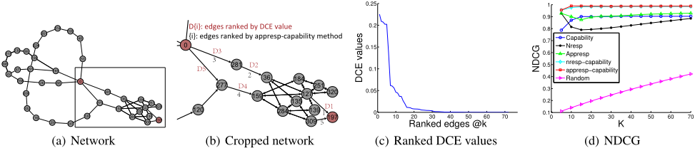
Figure 2: Causality based ranking of FB-Sample. The source node is 0, and the target node is 197. A directed edge stands for a directed message propagation between two nodes. (a) Network constructed by the traces in FB-Sample; (b) Cropped version of the network; (c) Ranked DCE values of all participant edges; (d) NDCG.
| source!target | #edges | #traces | Len(trace) | |
|---|---|---|---|---|
| FB-Sample | 0 ! 197 | 72 | 442 | 4 ⇠ 21 |
| FB-Walk-0-197 | 0 ! 197 | 1052 | 349 | 1 ⇠ 18 |
| FB-Walk-158-146 | 158 146 | 1024 | 213 | 2 18 |
158 ! 146 1024
2 ⇠ 18
FB-Walk-0-197 (start node 0 and target node 197) and FBWalk-158-146 (start node 158 and target node 146) are two large propagation history datasets with different start nodes and target nodes. They are generated as follows: 1) we start lots of random walks from the source node in the raw network; and 2) we record a random walk path (as a propagation trace) if it reaches the target in a limited number of steps.
To obtain the ranking ground truth, we run randomized experiments to get DCE values on four servers (with 8 cores and 32GB memory) for 100⇠400 hours for each dataset. 3
Evaluation Metric. We use NDCG as the evaluation metric in our experiments. NDCG is a popular evaluation metric following two rules: (i) highly related edges are more useful than marginally relevant ones; and (ii) lower ranked edges are less valuable for users, since they are less likely to be examined. The NDCG value of a ranking list at a particular rank position n is defined as:
where reli is the graded rating of the i-th edge in the ranking list, and Zn is a normalization constant to make the perfect list obtain NDCG score of 1. Note DCE values are used as the graded ratings (¶reli♦) in all experiments.
Ranking Strategies. With the proposed two indicators, we compare the following six different ranking strategies.
- Capability: Ranking by capability value (Section 4.2);
- Appresp: Ranking by responsibility value calculated by Appresp (Section 5);
- Nresp: Ranking by responsibility value calculated by Nresp [Qin et al., 2013];
3 To get convergent values, we have to conduct randomized experiments with lots of repetitions (around 109 ). Moreover, larger propagation history datasets need even more repetitions.
- appresp-capability: The integrated "resp-cap" ranking (Section 4.3) with responsibility calculated by Appresp;
- nresp-capability: The integrated "resp-cap" ranking (Section 4.3) with responsibility calculated by Nresp;
- Random: Ranking randomly.
In the integrated "resp-cap" methods, we all set the parameter ↵=0▷5. For each method, we first get the ranking list. Then, we generate 1000 permutations of this list by shuffling edges with the same ranking score. Finally, we use the mean NDCG of these permutations as this method's performance.
6.2 Ranking Quality
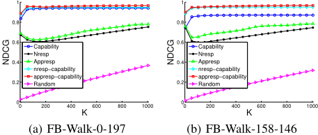
(1) ComparingQuality. We evaluate the six ranking strategies. Figures 2(d) and 3 show the experimental results. Table 2 shows the details. In addition, we show the top-5 ranked edges obtained by DCE values and our appresp-capability method in Fig. 2(b). Due to space limitations, we only show the top ranked edges on FB-Sample, but the results are similar on the other two datasets.
Our first observation is that our integrated ranking methods (appresp-capability and nresp-capability) successfully capture the intuition of DCE. As shown in Fig. 2(b), our appresp-capability method successfully identifies the top important edges in the propagation history. The nresp-capability method could do the same thing (we do not show it, due to space limitations). Therefore, our integrated methods achieve a high ranking accuracy. Take NDCG@5 as an example, integrated methods get a ranking accuracy of 90⇠95%.
Our second observation is that our integrated ranking methods significantly outperform unintegrated ones. Take
261
314
199
48
| FB-Sample | FB-Walk-0-197 | FB-Walk-158-146 | |||||||
|---|---|---|---|---|---|---|---|---|---|
| Method | NDCG@5 | NDCG@10 | NDCG@15 | NDCG@5 | NDCG@10 | NDCG@15 | NDCG@5 | NDCG@10 | NDCG@15 |
| Capability | 0.7870 | 0.8703 | 0.9009 | 0.8354 | 0.8476 | 0.8726 | 0.7442 | 0.7083 | 0.7319 |
| Nresp | 0.9274 | 0.8143 | 0.7900 | 0.6706 | 0.7417 | 0.7933 | 0.7435 | 0.7758 | 0.7122 |
| Appresp | 0.9277 | 0.9004 | 0.8739 | 0.6872 | 0.7579 | 0.8061 | 0.7575 | 0.7903 | 0.7311 |
| nresp-capability | 0.9548 | 0.9762 | 0.9827 | 0.8769 | 0.9019 | 0.9100 | 0.8900 | 0.9369 | 0.9146 |
| appresp-capability | 0.9549 | 0.9892 | 0.9889 | 0.8871 | 0.9213 | 0.9291 | 0.9004 | 0.9534 | 0.9303 |
| Random | 0.1110 | 0.1405 | 0.1682 | 0.0277 | 0.0299 | 0.0310 | 0.0165 | 0.0194 | 0.0223 |
NDCG@5 as an example, integrated ones outperform unintegrated ones by 10⇠25%. This improvement persists even when the rank position increases Therefore, both the first and second observations demonstrate that our integrated strategy can capture two faces of causal effects and thus improve the performance by combining these two indicators. This summary answers the aforementioned question Q2.
The last observation is that ranking either by capability or by responsibility (Appresp or Nresp) alone can achieve a passable accuracy. Take NDCG@5 as an example, the ranking accuracies of unintegrated ones are around 75%. This is consistent with our theoretical analysis that responsibility and capability can evaluate causal contribution in two different faces. This answers the aforementioned question Q1.
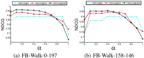
(2) The Effect of Parameter ↵. In our integrated "resp-cap" ranking strategy, there is a parameter ↵ balancing consideration of causation between necessity and sufficiency. We test different values of ↵ in this kind of method on two large propagation history datasets. Figure 4 shows the results. We can see that 1) combining appresp and capability values does increase ranking performance; and 2) although the results fluctuate, the performances with ↵ around 0▷5 are always stable and preferred. These observations suggest that we should consider the necessity and sufficiency of causation fairly.
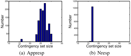
(3) Appresp vs. Nresp. We also compare two responsibility calculation methods: Appresp and Nresp. From Figs. 2(d) and 3, we can see that Appresp outperforms Nresp in both the unintegrated and integrated strategies. We can explain this from Fig. 5, which shows the size distributions of the contingency sets calculated by these two methods. (We report only the result on FB-Walk-0-197, because the results of the rest of networks show the same trend.) The results of Nresp are highly centralized, which indicates the results are highly influenced by those edges involved in more traces. In contrast, the results of Appresp are decentralized. This is because Appresp could guarantee a feasible result, so as to avoid being highly affected by the edges with large influence.
7 RelatedWork
Causality. The classical counterfactual causality (if X had not occurred, Y would not have occurred) goes back to [Hume, 1739]. [Lewis, 1973] analyzed it in a formal way. Recently, [Pearl, 2000] has given a rigorous definition of causality. Under this definition, [Chockler and Halpern, 2004] introduced responsibility to evaluate the contribution of each cause. [Meliou et al., 2010a; Freire et al., 2015] studied the causality and responsibility problems in relational databases. We refer to [Kleinberg and Hripcsak, 2011] and [Li et al., 2015] for expositions of causality theory.
Diffusion in SNS. Understanding information diffusion is one of the primary reasons for studying SNS [Guille et al., 2013]. This topic has many interesting applications, such as influential spreaders identification [Kitsak et al., 2010], influence maximization [Chen et al., 2015], and hot topic identification [Kleinberg, 2003]. Most of them analyzed diffusion problems based on the network structure.
In this paper, we analyze diffusion based on propagation histories rather than network structure. In addition, we propose to understand the diffusion from the viewpoint of causality, which has rarely been mentioned in the literature.
8 Conclusion
This paper presents the propagation history ranking problem in SNS, and puts forward a solution from the viewpoint of causality. We first introduce DCE as the ranking criterion and show its rationality. Due to the hardness of calculating DCE, we then propose the "resp-cap" ranking strategy by adopting two indicators (responsibility and capability). Furthermore, we design an approximate algorithm for responsibility calculation, which could guarantee a feasible solution for general propagation histories. Extensive experiments demonstrate the feasibility and advantages of our approach. As future work, we would like to consider more complicated diffusion.
Acknowledgments
This work is supported in part by the National Natural Science Foundation of China (No. 61373023, No. 61170064) and NSF through grants III-1526499.
@inproceedings{ijcai2016p551,
  title     = {Causality Based Propagation History Ranking in Social Networks},
  author    = {Wang, Zheng and Wang, Chaokun and Pei, Jisheng and Ye, Xiaojun and Yu, Philip S.},
  booktitle = {Proceedings of the Twenty-Fifth International Joint Conference on
               Artificial Intelligence, {IJCAI-16}},
  publisher = {AAAI Press / International Joint Conferences on Artificial Intelligence},
  editor    = {Subbarao Kambhampati},
  pages     = {3917--3922},
  year      = {2016},
  month     = {7},
  url       = {https://ijcai.org/proceedings/2016/551},
}
TY - CPAPER TI - Causality Based Propagation History Ranking in Social Networks AU - Wang, Zheng AU - Wang, Chaokun AU - Pei, Jisheng AU - Ye, Xiaojun AU - Yu, Philip S. T2 - Proceedings of the Twenty-Fifth International Joint Conference on Artificial Intelligence, IJCAI-16 PB - AAAI Press / International Joint Conferences on Artificial Intelligence PY - 2016 SP - 3917 EP - 3922 UR - https://ijcai.org/proceedings/2016/551 ER -Copied
Machine-readable versions of this paper, for tools and AI agents:





