
Catcher-Evader Games
Proceedings of the Twenty-Fifth International Joint Conference on Artificial Intelligence. Pages 329-336.
© 2016 International Joint Conferences on Artificial Intelligence
Abstract
Algorithms for computing game-theoretic solutions have recently been applied to a number of security domains. However, many of the techniques developed for compact representations of security games do not extend to Bayesian security games, which allow us to model uncertainty about the attacker's type. In this paper, we introduce a general framework of catcher-evader games that can capture Bayesian security games as well as other game families of interest. We show that computing Stackelberg strategies is NP-hard, but give an algorithm for computing a Nash equilibrium that performs well in experiments. We also prove that the Nash equilibria of these games satisfy the interchangeability property, so that equilibrium selection is not an issue.
- [An et al., 2012] Bo An, Eric Shieh, Milind Tambe, Rong Yang, Craig Baldwin, Joseph DiRenzo, Ben Maule, and Garrett Meyer. PROTECT -A deployed game theo- retic system for strategic security allocation for the United States Coast Guard. AI Magazine, 33(4):96-110, 2012.
- [Birkhoff, 1946] Garrett Birkhoff. Tres observaciones sobre el algebra lineal. Univ. Nac. Tucumn Rev, Ser. A, no. 5, pages 147-151, 1946.
- [Borie et al., 2009] Richard B Borie, Craig A Tovey, and Sven Koenig. Algorithms and complexity results for pursuit-evasion problems. In IJCAI, volume 9, pages 59- 66, 2009. IJCAI
- [Kiekintveld et al., 2009] Christopher Kiekintveld, Manish Jain, Jason Tsai, James Pita, Fernando Ordóñez, and Milind Tambe. Computing optimal randomized resource allocations for massive security games. In Proceedings of the Eighth International Joint Conference on Autonomous Agents and Multi-Agent Systems (AAMAS), pages 689- 696, Budapest, Hungary, 2009.
- [Korzhyk et al., 2010] Dmytro Korzhyk, Vincent Conitzer, and Ronald Parr. Complexity of computing optimal Stack- elberg strategies in security resource allocation games. In Proceedings of the National Conference on Artificial Intel- ligence (AAAI), pages 805-810, Atlanta, GA, USA, 2010.
- [Korzhyk et al., 2011a] Dmytro Korzhyk, Vincent Conitzer, and Ronald Parr. Security games with multiple attacker resources. In Proceedings of the Twenty-Second Interna- tional Joint Conference on Artificial Intelligence (IJCAI), pages 273-279, Barcelona, Catalonia, Spain, 2011. IJCAI
- [Korzhyk et al., 2011b] Dmytro Korzhyk, Zhengyu Yin, Christopher Kiekintveld, Vincent Conitzer, and Milind Tambe. Stackelberg vs. Nash in security games: An extended investigation of interchangeability, equivalence, and uniqueness. Journal of Artificial Intelligence Re- search, 41(2):297-327, 2011.
- [Li and Conitzer, 2013] Yuqian Li and Vincent Conitzer. Game-theoretic question selection for tests. In Proceed- ings of the Twenty-Third International Joint Conference on Artificial Intelligence (IJCAI), pages 254-262, Beijing, China, 2013. IJCAI
- [Parsons, 1978] Torrence D Parsons. Pursuit-evasion in a graph. In Theory and applications of graphs, pages 426- 441. Springer, 1978.
- [Paruchuri et al., 2008] Praveen Paruchuri, Jonathan P. Pearce, Janusz Marecki, Milind Tambe, Fernando Ordóñez, and Sarit Kraus. Playing games for security: An efficient exact algorithm for solving Bayesian Stackelberg games. In Proceedings of the Seventh International Joint Conference on Autonomous Agents and Multi-Agent Systems (AAMAS), pages 895-902, Estoril, Portugal, 2008.
- [Pita et al., 2009a] James Pita, Manish Jain, Fernando Ordóñez, Christopher Portway, Milind Tambe, and Craig Western. Using game theory for Los Angeles airport secu- rity. AI Magazine, 30(1):43-57, 2009.
- [Pita et al., 2009b] James Pita, Manish Jain, Fernando Ordóñez, Christopher Portway, Milind Tambe, Craig Western, Praveen Paruchuri, and Sarit Kraus. Using game theory for Los Angeles airport security. AI Magazine, 30(1):43-57, 2009.
- [Tsai et al., 2009] Jason Tsai, Shyamsunder Rathi, Christo- pher Kiekintveld, Fernando Ordóñez, and Milind Tambe. IRIS -A tool for strategic security allocation in trans- portation networks. In Proceedings of the Eighth Interna- tional Joint Conference on Autonomous Agents and Multi- Agent Systems (AAMAS), pages 37-44, Budapest, Hun- gary, 2009.
- [Yin et al., 2012] Zhengyu Yin, Albert Xin Jiang, Milind Tambe, Christopher Kiekintveld, Kevin Leyton-Brown, Tuomas Sandholm, and John P. Sullivan. TRUSTS: Scheduling randomized patrols for fare inspection in tran- sit systems using game theory. AI Magazine, 33(4):59-72, 2012.
References were extracted automatically from the PDF and may contain errors.
Full text extracted automatically from the PDF; figures, tables and equations may differ. The PDF is the version of record.
1 Introduction
Algorithms for computing game-theoretic solutions have long been of interest to AI researchers. In recent years, applications of these techniques to security have drawn particular attention. These applications include airport security [Pita et al., 2009a], the assignment of Federal Air Marshals to flights [Tsai et al., 2009], scheduling Coast Guard patrols [An et al., 2012], scheduling patrols on transit systems [Yin et al., 2012], and the list goes on. Game-theoretic techniques are natural in these domains because they involve parties with competing interests (though the games are usually not zerosum), and the use of mixed (randomized) strategies to avoid being predictable to one's opponent is desirable.
These applications have typically used a Stackelberg model where one player (the defender) commits to a mixed strategy first and the other (the attacker) then optimally responds to this mixed strategy. Formally, the defender (player 1) chooses a mixed strategy σ⇤ 1 2 argmaxσ1 maxs22BR2 (σ1) u1(σ1↪ s2), 1 where BR2 (σ1) is the set of best responses to σ1 for player 2 (i.e., the responses that maximize player 2's utility). This is in contrast to the more standard solution concept of Nash equilibrium, where both players play a mixed strategy in such a way that each plays a best response to the other-that is, a pair (σ1↪ σ2) with σ1 2 BR1 (σ2) and σ2 2 BR2 (σ1). Arguably, the Stackelberg solution is well motivated in contexts where the attacker can learn the defender's strategy over time by repeated observation, whereas if this is not the case perhaps the Nash solution is better motivated. It is known that under certain conditions in security games, Stackelberg strategies are also Nash equilibrium strategies [Korzhyk et al., 2011b].
⇤The full version of this paper is available at http://arxiv.org/abs/1602.01896. Dmytro contributed to this paper while he was a Ph.D. student at Duke University.
1 Generally, if the attacker is indifferent among multiple targets, the defender can slightly modify her strategy to make any one of
Initial work in these domains modeled uncertainty over attacker preferences using the formalism of Bayesian games, assigning probabilities to different types of attackers. This included the original work at the airport at Los Angeles [Paruchuri et al., 2008]. However, subsequent research, which started to focus on compact representations of security games, mostly did not consider Bayesian games. In this paper, we introduce a more general framework that can capture such Bayesian security games, and study the computation of Stackelberg and Nash solutions in them (which in such games generally do not coincide). Our framework can also model certain types of test games in which a tester randomly chooses questions from a fixed database of questions [Li and Conitzer, 2013]. We show that computing a Stackelberg strategy is strongly NP-hard, but give an algorithm for computing Nash equilibria that combines and expands on earlier techniques in both security and test games. While we have been unable to show that our algorithm is guaranteed to require at most polynomially many iterations, it requires few iterations in experiments.
More benefits of our framework are listed below: (1) Our notation for Catcher-Evader 2 games, once one becomes familiar with it, greatly simplifies analysis of those games, especially as it concerns utilities. For example, our notation expresses the utility delta of a target, which is often the crucial quantity, directly as d, rather than as a difference (e.g., uci - uui ). (2) Our additional parameters a↪ b↪ c allow richer utility functions that security games did not capture previously. For example, targets may have different costs to defend even if the attacker does not attack them. Previous security game definitions always assumed no cost (or the same cost) if the attacker does not attack. (3) It lets us swap the roles of defenders and attackers. Therefore, we can also directly compute the attacker's strategy as well as the defender's strategy, an example of which is computing the tester's strategy in test games. (4) Its connection between security games and test games brings enormous convenience for algorithm design. Previously, separate algorithms had to be designed for them, but now we can design a single algorithm for both. Moreover, we can potentially apply known algorithms for each of these game families to the other. For example, the aforementioned Nash equilibria algorithm combines techniques for security games (progressively increasing defender or catcher resources) and test games (using network flow to reallocate attacker or evader resources). (5) Besides security games and test games, it can also capture other interesting scenarios where resources must be assigned to different targets by two competing parties. For example, two companies, an incumbent and an entrant, might be allocating capital to different markets; the entrant may wish to evade the incumbent and build up market share, while the incumbent wants to catch the entrant to drive the latter out of business.
these uniquely optimal; this is why ties for the attacker are broken in favor of the defender.
2 Note that these games are completely different from pursuitevasion (or cops-and-robbers) games [Parsons, 1978; Borie et al., 2009]. Those games involve dynamically chasing another player on a graph. Our games, in contrast, occur in a single period, and concern the computation of an optimal random assignment.
2 Notation
We model a Catcher-Evader game (CE game) as a game between one catcher and multiple evaders. Since we assume that the evaders do not care about each other's actions, this is equivalent to a Bayesian game between a single-typed catcher and an evader with multiple types. Also, as we will show in section 3.3, the roles of catcher and evader can be swapped. Hence, our model also captures games between one evader and multiple catchers.
We represent a CE game by (N↪ ↪ r↪ `↪ a↪ b↪ c↪ d), where N = ¶0↪ 1↪ ▷ ▷ ▷ ↪ n♦ is the set of players and is the set of sites (e.g., the targets in a security game or the questions in a test game). We fix 0 2 N to be the catcher (e.g., the defender in a security game), and N + = ¶1↪ 2↪ ▷ ▷ ▷ ↪ n♦ to be the set of evaders (e.g., the multiple types of attackers in a security game). Player i 2 N has available a total resource amount of ri 2 R≥0 . For example, we might set ri = 1 to indicate that i has only one resource, or we might set ri = 1◁2 to indicate that, in a Bayesian game, a type i that appears with probability 1◁2 has only a single resource, and therefore the expected number of resources that this type contributes is 1◁2. This resource amount can be split fractionally across the sites, for example, 1◁3 could be assigned to one site and 2◁3 to another. (This would typically correspond to assigning a single resource to the former site with probability 1◁3.) Player i can assign a resource amount of at most `i↪ 2 R to site 2 . For example, we might set `i↪ = 1 to indicate that i can assign at most a single resource to , or we might set `i↪ = 1◁2 to indicate that, in a Bayesian game, a type i that appears with probability 1◁2 can assign at most a single resource to if he appears, and therefore his marginal contribution of probability mass to is at most 1◁2. Generally, ri P 2 `i↪ so the player has to make a nontrivial decision about which site gets more of the resource amount and which one gets less.
Finally, the utility is encoded by a↪ b↪ c↪ d as follows. Let x be the strategy profile where xi↪ is the resource amount that player i puts on site . For convenience, we denote x⌃↪ = Pni=1 xi↪ as the combined resource amount that all n evaders put on site . Then the utility is P 2 [(b0↪ +d0↪ x⌃↪ )x0↪ +a0↪ x⌃↪ + c0↪ ] for the catcher and P 2 [(bi↪ +di↪ x0↪ )xi↪ +ai↪ x0↪ + ci↪ ] for evader i. Here, b is the base utility for a player to put a resource at a site, and d is the utility change that results from putting a resource at that site when the opponent puts a resource there as well. Since c (constant utility) is not affected by any player's strategy, we can ignore it (or let c = 0) without affecting our analysis of both Stackelberg strategies and Nash equilibrium. Finally, a (for alternating utility) is the utility that a player receives when the opponent puts a resource at that site; the former player cannot affect this. Hence, for Nash equilibrium (but not for Stackelberg strategies), we can simply drop a (or let a = 0). We require P 2 xi↪ = ri for feasibility, as well as d0↪ > 0 and di↪ < 0 for i 2 N + so that the catcher wants to catch the evader while the evader wants to evade.
For convenience, we define x-0↪ = x⌃↪ and x-i↪ = x0↪ for i 2 N +. Then, we define θi↪ = (bi↪ + di↪ · x-i↪ ) as the per-resource utility of player i on site . That is, it is the increase in utility she experiences from putting one more resource there. So, player i's utility gained from site can be written as ui↪ (x) = θi↪ xi↪ + ai↪ x-i↪ + ci↪ . In a best-response strategy, player i should have a utility threshold ✓i such that (1) for all with θi↪ (x) > ✓i, the player maximizes the resource amount it puts there (xi↪ = `i↪ ), and (2) for all with θi↪ (x) < ✓i, the player puts no resource amount there (xi↪ = 0). (There is no requirement for the case θi↪ (x) = ✓i.) The value of ✓i is not necessarily unique, so for definiteness, let ✓0 = max 2 :x0↪ <`0↪ θ0↪ and ✓i =min 2 :xi↪ >0 θi↪ for i 2 N +.
In Table 1, we summarize all symbols for reference.
Incidentally, note that if we do not require d0↪ > 0 and di↪ < 0 for i 2 N +, then a↪ b↪ c↪ d can represent any utility function of the form P 2 f(xi↪ ↪ x-i↪ ) where f is a quadratic polynomial without factors x2i↪ or x2-i↪ .
3 Reducing Games to CEGames
In this section, we show how the framework of CE games let us capture several game families studied previously in the literature, namely security games and test games.
3.1 Security Games
A general definition of security games was given by [Kiekintveld et al., 2009]. That work considered only a single attacker resource; an attacker with multiple attacker resources was considered by [Korzhyk et al., 2011a]. More generally still, we can consider a Bayesian game in which there is uncertainty about the type of the attacker. (Some of the earliest work in this line of research concerned Bayesian games [Paruchuri et al., 2008; Pita et al., 2009b], but the games were relatively small and so the techniques did not exploit the structure of security games.) We now define multiresource Bayesian security games and show how to reduce them to CE games. Note that in our definition, a resource is assigned to a single target. 3
| Description |
| N Set of players ¶0↪ 1↪ ▷ ▷ ▷ ↪ n♦ + |
| N Evaders ¶1↪ 2↪ ▷ ▷ ▷ ↪ n♦ (0 is the catcher) |
| Set of sites (e.g., targets in security games) |
| ri Resource of player i |
| `i↪ Resource limit player i can put on site |
| ai↪ Alternating utility of player i on site |
| bi↪ Base utility of player i on site |
| ci↪ Constant utility of player i on site |
| di↪ Utility change (delta) of player i on site |
| xi↪ Amount of resource i puts on (strategy) |
| x⌃↪ Sum of all evaders' resource on |
| x-i↪ Amount of resource i's opponent puts on |
| θi↪ Per-resource utility of i on : bi↪ +di↪ x-i↪ |
| ui↪ Utility of i on : θi↪ xi↪ +ai↪ x-i↪ + ci↪ ✓i Utility threshold of player i |
There are a defender and an attacker. The latter has unknown type i 2 ¶1↪ ▷ ▷ ▷ ↪ n♦. An attacker of type i occurs with probability pi. There are m targets t1↪ t2↪ ▷ ▷ ▷ ↪ tm. An attacker of type i can attack ri distinct targets while the defender can defend rd distinct targets. A player's utility is the sum of its utility over all targets. If an attacker of type i attacks an undefended target t, it obtains utility uui (t) (and the defender obtains utility uud (t)). If it attacks a defended (covered) target t, it obtains utility uci (t) (and the defender obtains utility ucd (t)). Both players obtain utility 0 from t if t is unattacked.
Now, we can reduce this to the following CE game (N↪ ↪ r0 ↪ a0 ↪ b0 ↪ c0 = 0↪ d0 ) (see Table 2 for an example of utility reduction): N = ¶0↪ 1↪ 2↪ ▷ ▷ ▷ ↪ n♦↪ = ¶t1↪ t2↪ ▷ ▷ ▷ ↪ tm♦↪ r00 = rd↪ r0i = piri (i 2 N +)↪ `00↪ = 1↪ `0i↪ = pi ( 2 ↪ i 2 N +)↪ a00↪ = uud ( )↪ b00↪ = 0↪ d00↪ = ucd ( ) - uud ( )↪ a0i↪ = 0↪ b0i↪ = uui ( )↪ d0i↪ = uci ( ) -uui ( ) (i 2 N +).
Note that in the original security game, r consists of natural numbers and a pure strategy would put either 0 or 1 resources on each site. In the CE game, the strategy profile xi↪ corresponds to the marginal probability that player i puts a resource on . Because resources can only be assigned to single targets, we can always use Birkhoff-von Neumann decomposition [Birkhoff, 1946] to generate a valid mixed strategy of the original security game with these marginals (see also [Korzhyk et al., 2010]).
3 Section 6 of [Kiekintveld et al., 2009] also allowed resources to be assigned to schedules of multiple targets, which quickly leads to NP-hardness [Korzhyk et al., 2010].
| Player | Security Game | CE Game | ||||
|---|---|---|---|---|---|---|
| uci (t) | uui (t) | ai↪t | bi↪t | ci↪t | di↪t | |
| Def (i = 0) | 1 | -10 | -10 | 0 | 0 | 11 |
| Att 1 (i = 1) | -5 | 5 | 0 | 5 | 0 | -10 |
| Att 2 (i = 2) | -9 | 10 | 0 | 10 | 0 | -19 |
3.2 Testing Games
Testing games were recently studied by [Li and Conitzer, 2013]. In that work, only test takers that do not fail any questions pass the test; therefore, it does not matter whether a test taker fails 1 question or 100. In contrast, we consider a variant-arguably more realistic-in which the losses and gains the players experience are additive across questions. We call this variant "scored tests", which captures cases like the GRE, the TOEFL, and most course exams at school. It allows us to bypass the (co)NP-hardness results for computing the best test strategies from [Li and Conitzer, 2013]. On the other hand, the transformation to a zero-sum game described in that paper no longer works in this context.
Formally, a test game is a 2-player game between a tester and a test taker. The tester is uncertain about the test taker's type i 2 ¶1↪ 2↪ ▷ ▷ ▷ ↪ n♦, but she knows that a test taker of type i occurs with probability pi. The tester has a pool of questions Q, from which t questions will be chosen to form a test T ✓ Q (♣T ♣ = t). For a test taker of type i, a given subset Hi ✓ Q of questions are hard and he will not be able to solve them unless he memorizes their answers (or writes them on a cheat sheet). However, he can memorize at most m✓ questions, so if the tester randomizes over the choice of T, there is a good chance that most questions in T have not been memorized. We denote the set of questions i chooses to memorized as Mi ✓ Q(♣Mi♣ = mi)
So far, everything is identical to the games defined by [Li and Conitzer, 2013]. Now we introduce a question score sq for each q 2 Q. If a test taker fails to solve q in the test, sq is deducted from his score. Hence the test taker's utility is ui(T↪Mi) = - Pq2T\Hi∩Mi sq. 4 We also introduce a weight wq for each question, representing how important the tester thinks it is to find out whether the test taker can solve q. This may or may not be equal to sq. The tester's utility is then uti (T↪Mi) = vi Pq2T\Hi∩Mi wq. Here, vi denotes the tester's assessment of the importance of test taker type i. For example, it might be more (or less) important to figure out the true score of a bad test taker (with large Hi) than that of a good one. We reduce this game to the CE game (N↪ ↪ r↪ a↪ b↪ c = 0↪ d) where N = ¶0↪ 1↪ 2↪ ▷ ▷ ▷ ↪ n♦↪ = Q↪ r0 = t↪ ri = pivimi (i 2 N +)↪ `0↪q = 1↪ `i↪q = pivi (i 2 N +↪ q 2 Q = )↪ a0↪q = 0↪ b0↪q = wq Pi:q2Hi pivi↪ d0↪q = -wq↪ ai↪q = -sq for q 2 Hi↪ ai↪q = 0 for q ◁2 Hi↪ bi↪q = 0 (i 2 N +)↪ di↪q = sq◁ri↪q for q 2 Hi↪ di↪q = 0 for q ◁2 Hi.
4 A constant Pq2T sq can be added to ui(T↪Mi) to obtain the usual nonnegative test scores.
(a) An example of test game players' utility on a question q
| test taker's utility, tester's utility | don't test q | test q |
| don't memorize q | 0, 0 | -5, 4 |
|---|---|---|
| memorize q | 0, 0 | 0, 0 |
(b) Swapping roles for the above example test game
| Player | ai↪q | bi↪q | ci↪q | di↪q | |
|---|---|---|---|---|---|
| test q: | Tester (i = 0) | 0 | 4 | 0 | -4 |
| x0↪q = 1 | Test taker (i = 1) | -5 | 0 | 0 | 5 |
| test q: | Tester (i = 0) | -4 | -4 | 4 | 4 |
| x0↪q = 0 | Test taker (i = 1) | 5 | 5 | -5 | -5 |
Similar to security games, the resulting strategy profile xi↪q denotes the marginal probability that a player puts q on the test / memorizes q; again, the Birkhoff-von Neumann theorem allows us to obtain a strategy with these marginals.
3.3 Swapping Roles
The reduction from test games has one issue: the utilities change at rates d0 < 0↪ di > 0 (i 2 N +) but CE games require d0 > 0↪ di < 0 (i 2 N +). In a sense, the tester is an evader who wants to evade by asking questions that are not memorized by the test taker; but as we have defined them, in CE games, player 0 is a catcher.
We handle this by redefining player 0's resources to their opposites. That is, we focus on which questions she does not test. Hence, the modified x00↪q will be the marginal probability that she does not test q (i.e., q ◁2 T).
In general, we can swap roles between catchers and evaders (i.e., negate d) by rewriting CE game (N↪ ↪ r↪ a↪ b↪ c↪ d) as CE game (N↪ ↪ r0 ↪ a0 ↪ b0 ↪ c0 ↪ d0 ): r00 = -r0 + P 2 `0↪ ↪ r0i = ri (i 2 N +)↪ `0i↪ = `i↪ (i 2 N)↪ a00↪ = a0↪ + d0↪ `0↪ ↪ c00↪ = c0↪ + b0↪ `0↪ ↪ b00↪ = -b0↪ ↪ d00↪ = -d0↪ ↪ a0i↪ = -ai↪ ↪ d0i↪ = -di↪ ↪ b0i↪ = bi↪ +di↪ `0↪ ↪ c0i↪ = ci↪ +ai↪ `0↪
Hence, the utilities are exactly the same as in the original game. As previously mentioned, c does not affect our gametheoretic analysis. However, it is essential for establishing these equations so we can swap roles. Of course, after the transformation, we can freely drop c0 . Table 3 shows an example of a test game and how we swap roles in it.
4 Complexity of Stackelberg Strategies
Theorem 1. If there is only one evader who can put all resources on any single site (8 2 ↪ `1↪ ≥ r1), then catcher Stackelberg strategies can be computed in polynomial time.
The proof of Theorem 1 (in the full version of this paper) uses a by now fairly standard linear program technique.
In contrast, it has been shown that computing Stackelberg strategies in a multi-resource security game (even with only a single type, i.e., non-Bayesian) is (weakly) NP-hard [Korzhyk et al., 2011a]. Hence, by our reduction of such security games to CE games, even if the CE game has only one evader (n = 1), it is (weakly) NP-hard to compute Stackelberg strategies if we allow `1↪ < r1 (so the evader/attacker will put resources on multiple sites).
Next, we show that even if `i↪ ≥ ri for all i ≥ 1, it is strongly NP-hard to compute Stackelberg strategies if we allow n > 1. This corresponds to the case of a Bayesian security game in which each attacker has only a single resource. Note that the initial LAX airport paper [Paruchuri et al., 2008] assumed a Bayesian security game with a single attacker resource. To our best knowledge, no hardness result has been given for computing Stackelberg strategies of such games. Also, unlike the known weak NP-hardness result for multiple resources, this rules out pseudopolynomial-time algorithms. The proof is in the full version of this paper to save space.
Theorem 2. Computing Stackelberg strategies in Bayesian security games is strongly NP-hard even if each attacker type has only a single resource. Consequently, computing Stackelberg strategies in a Catcher-Evader game is strongly NP-hard (if n > 1), even if `i↪ ≥ ri for all i 2 N +. (This result is tight in the sense that this problem is also in NP.)
5 Interchangeability of NE
We now move on to studying Nash equilibria. In general, a downside of the Nash equilibrium concept is that Nash equilibria can fail interchangeability: if one player plays according to one Nash equilibrium and the other according to another, the result may not be a Nash equilibrium. However, it has been shown that interchangeability of Nash equilibria is guaranteed in security games and test games under certain conditions [Korzhyk et al., 2011b; 2011a; Li and Conitzer, 2013]. We now show that this also holds for CE games. The key lemma and theorem are shown below. Their proofs are in the full version to save space.
Lemma 1. For each site , either x0↪ is the same for all NE or x⌃↪ is the same for all NE.
Theorem 3. The Nash equilibria (NE) of a Catcher-Evader game are interchangeable. That is, if x and x0 are two Nash equilibrium strategy profiles, then so is x00 where x00 0↪ = x0↪ and x00 i↪ = x0i↪ (i 2 N +).
6 Computing Nash Equilibrium
The interchangeability established in the previous section provides good motivation for computing a Nash equilibrium in this domain. In this section, we provide an algorithm for doing so. The algorithm is significantly more involved than earlier algorithms, notably requiring a min-cost-flow subroutine. This is perhaps surprising as earlier algorithms-e.g., the one by [Korzhyk et al., 2011a] for computing a Nash equilibrium in non-Bayesian security games with multiple attacker resources-do not need to do so. However, in the next subsection, we show it is possible to reduce the problem of finding a minimum-cost fractional matching to our games, suggesting that this complexity is inherent in the problem. We have been unable to either give a polynomial upper bound on the number of iterations of our algorithm (each iteration takes polynomial time), or any class of instances that results in superpolynomially many iterations. We only give an exponential upper bound. However, as we will show, in experiments few iterations suffice.
6.1 Reducing fromMin-Cost Matching
We show that computing an NE in CE games (even with single-resource evaders, i.e., 8i 2 N +↪ `i↪ ≥ ri) is as hard as computing minimum-cost fractional 5 matchings-a common type of flow problem-suggesting that we are unlikely to find a linear-time algorithm. Some of the ideas in the reduction, in particular having costs in the graphs corresponding to the logarithms of utility change rates d, will also appear in the algorithmwe present later.
Theorem 4. Computing a Nash equilibrium of a CE game is as hard as computing a minimum-cost fractional matching of a weighted bipartite graph. Specifically, if there is a Nash equilibrium finding algorithm that runs in T(I) time, where I is the input size of the CE game, then we can solve the matching problem in T(O(I 0 )) time, where I 0 is the input size of the bipartite graph. So computing a NE is not possible in linear time unless there is a linear algorithm for matching.
Proof. We reduce the matching instance to a CE game whose NE can be straightforwardly translated back to an optimal solution to the matching instance. The reduction takes linear time, resulting in the bound in the theorem.
5 Of course, network flow problems have an integrality property-but not if the input is fractional, as we allow here.
Let the matching instance be on a bipartite graph with vertices U = ¶1↪ ▷ ▷ ▷ ↪ n♦ and V . Each vertex v has a capacity v, with Pu2U u = Pv2V v. Each edge (u↪ v) has a capacity (u↪ v) and a cost w(u↪ v). Our goal is to saturate all the vertices' capacities at minimum cost. Equivalently, this is a flow problem where Pu2U u flow must be pushed across the bipartite graph at minimum cost.
First, we note that the game has a feasible strategy for the evaders if and only if the matching problem has a feasible solution. This is because a feasible strategy xu↪v corresponds exactly to a feasible matching solution.
We construct a CE game (N↪ ↪ r↪ a↪ b↪ c = 0↪ d) where N = ¶0↪ 1↪ 2↪ ▷ ▷ ▷ ↪ n♦ (so N + = U), = V , r0 = 1 and ru = u for all u 2 U, `0↪v = 1 and `u↪v = (u↪ v) for all u 2 U and v 2 V , bi↪v = 0 for all i 2 N↪ v 2 V , d0↪v = 1◁v and du↪v = -ew(u↪v) for all u 2 U and v 2 V .
Second, x0↪v > 0 must hold for all v. Otherwise, because bu↪v = 0 and du↪v < 0, all evaders will strictly prefer targets with x0↪v = 0; but then the catcher would not be bestresponding, because b0↪v = 0 and d0↪v > 0.
Finally, we show that the NE x must constitute an optimal solution to the matching problem. That is, if we let W = Pu2U↪v2V xu↪vw(u↪ v) then W is the minimum cost in the matching problem. Suppose not; then, when interpreting xu↪v as a flow, in the residual graph of that flow, a negative cycle exists. Let that cycle be u1 ! v1 ! u2 ! v2 ! ▷ ▷ ▷ ! um ! vm ! u1 with P1km(w(uk↪ vk) - w(uk+1↪ vk)) < 0, xuk↪vk < (uk↪ vk), and xuk+1↪vk > 0 for all 1 k m (letting um+1 = u1). Recall that ✓u is the per-resource utility threshold for evader u. So, θuk↪vk = x0↪vk duk↪vk ✓uk and θuk+1↪vk = x0↪vk duk+1↪vk ≥ ✓uk+1 . Equivalently, x0↪vk ♣duk+1↪vk ♣ ♣✓uk+1 ♣ and ♣✓uk ♣ x0↪vk ♣duk↪vk ♣ because du↪v < 0. It then follows that
which implies Qmk=1 ♣duk+1↪vk ♣ Qmk=1 ♣duk↪vk ♣ because x0↪v > 0 for all v and thus ♣✓u♣ > 0 for all u 2 U. Taking the logarithm on both sides, we obtain P1km(w(uk↪ vk)- w(uk+1↪ vk)) ≥ 0, contradicting the negative cycle assumption P1km(w(uk↪ vk) - w(uk+1↪ vk)) < 0.
6.2 Algorithm
We now present our algorithm. The algorithm works by initializing the catcher's resource amount to 0 and gradually increasing it to r0, maintaining the equilibrium throughout. The same high-level approach was used by an earlier paper [Korzhyk et al., 2011a] for the case of a single attacker type (evader) with multiple resources, obtaining an efficient algorithm there. However, the case with multiple evaders is significantly more involved. The (polynomial-time) algorithm given in [Korzhyk et al., 2011a] did not require anything like a network-flow subroutine, whereas the reduction in section 6.1 suggests that this is necessary when we have multiple evaders. Our algorithm also incorporates ideas used in the context of test games [Li and Conitzer, 2013], specifically the binary search and max-flow techniques used there.
We first introduce some notation. Let Bi = ¶ ♣ θi↪ = ✓i♦ be the boundary sites of player i. Let B+ i = ¶ 2 Bi ^ xi↪ > 0♦ be evader i (i 2 N +)'s positive boundary sites, whose resource amount can be reduced. Let ˆB0 = ¶ 2 B0 ^ x0↪ < `0↪ ♦ be the catcher's open boundary sites, to which more resources could be assigned. Let the active edges be A = ¶(i↪ ) ♣ i 2 N +↪ 2 ↪ 2 Bi♦.
The main algorithm is Algorithm 1. After initializing, the algorithm repeatedly loops through Algorithms 2, 3, and 4, which together provably (eventually) increase the catcher's (allocated) resource amount while maintaining equilibrium. Algorithm 2 ensures that a "no negative cycle" property holds by solving a min-cost flow problem (since the residual flow of a min-cost flow cannot have a negative cycle). Here, the relationship between the evaders' best responses and the min-cost flow's "no negative cycle" property is similar to the reduction from min-cost matching that we gave earlier. Given that no negative cycle remains, Algorithm 3 then attempts to increase the catcher's resource amount-that is, for each it attempts to increase x0↪ -without breaking the evaders' bestresponse conditions. However, Algorithm 3 can still fail to increase the catcher's resource amount even without negative cycles. If so, we call Algorithm 4, which will either allow the next run of Algorithm 3 to strictly increase the catcher's resource amount, or change the open boundary sites ˆB0 (which provably cannot happen too often). Specifically, if Algorithm 3 failed to increase the catcher's resource amount, we have to reroute evaders' resources among their best-response sites, in a way that strictly decreases the catcher's utility threshold ✓0. Such rerouting must also maintain the catcher's best-response condition. For this we use max-flow and binary search: first, we binary search on ∆ , the decrease in ✓0; then, we calculate each edge's rerouting capacity using ∆, and see whether a max-flow can saturate all capacities, thereby maintaining the best-response condition.
Lemma 2. Algorithm 2 maintains Nash equilibrium without changing θi↪ or ✓i for any i 2 N + and 2 . As a result, the active edges A are also unchanged.
Proof. Algorithm2 only reallocates xi↪ amongA, hence the evaders necessarily continue to best respond. Both the original flow and the min-cost flow are required to saturate all edges ( ↪ ⌧). Hence x⌃↪ is unchanged for all 2 and the catcher necessarily continues to best respond. Each evader i's θi↪ is clearly unchanged as x0↪ is untouched by Algorithm2. By the definition of ✓i =min :xi↪ >0 θi↪ , the set of positive boundary sites B+ i must be non-empty, which means P 2Bi xi↪ > 0. So no matter how we reallocate, some 2 Bi must remain positive. Hence, ✓i is unchanged because the θi↪ are unchanged.
Lemma 3. In Algorithm 3, the evaders' thresholds ✓i (i 2 N +) decrease at rate γi. That is, the algorithm decreases ✓i by ∆ · γi.
We omit the proof of Lemma 3 to save space.
Lemma 4. After Algorithm 2, if Algorithm 3 successfully increases x0↪ , it maintains Nash equilibrium.
Proof. The catcher's strategy remains a best response because Algorithm 3 does not change any evader's strategy and the catcher only increases x0↪ for which θ0↪ = ✓0. Thus we only have to check whether each evader's strategy remains a best response.
By Lemma 3 and the notation θ0 ↪ ✓0 ↪A0 defined in its proof, evaders are best-responding if and only if:
For (i↪ ) ◁2 A0 , line 25 of Algorithm 3 maintains the conditions above. Now consider (i↪ ) 2 A0 . There, we have θ0i↪ = ✓0 i , so we only need to check
If xi↪ > 0, a backward edge ( ↪ i) with weight -w(i↪ ) exists in the residual graph. Hence dist(i) dist( ) - w(i↪ ), which implies -e-(dist( )-w(i↪ )) ≥ -e-dist(i) . That is, γ di↪ ≥ -γi, and therefore ∆ · γ · di↪ ≥ -∆ · γi because ∆ ≥ 0.
If xi↪ < `i↪ , a forward edge (i↪ ) with weight w(i↪ ) exists in the residual graph. Hence dist( ) dist(i) + w(i↪ ), which implies -e-(dist( )-w(i↪ )) -e-dist(i) .
That is. γ di↪ -γi, and therefore ∆· γ · di↪ -∆· γi because ∆ ≥ 0, completing the proof.
Lemma 5. If Algorithm 3 fails, then Algorithm 4 strictly decreases ✓0 while maintaining Nash equilibrium.
Proof. If Algorithm 3 fails, then for each 2 ˆB0, there must be another site 0 2 reachable \ unincreasable. That is, for each site 2 ˆB0 to which the catcher could increase resource assignment, there is a path in the residual graph that goes from to some site 0 2 unincreasable to which the catcher cannot increase resource assignment.
That site 0 is, in contrast, a good site for evaders: if they put more resources there, the catcher cannot penalize them (because the catcher cannot increase its resources there). Formally, there are two cases for 0 : 1) x0↪ 0 = `0↪ 0 ; 2) x0↪ 0 < ✓0. In the former case, evaders can increase their resource assignment there as much as possible because the catcher has hit the limit of what it can assign there. In the latter case, evaders can increase until θ0↪ 0 meets ✓0.
Therefore, for each 2 ˆB0, evaders can move a positive amount of resource from that site to some 0 ◁2 B0 using the corresponding residual graph path. The evaders continue to best-respond because the residual graph only includes active edges A. The catcher's best-response condition is maintained by decreasing θ0↪ by the same positive amount ∆ (the number found by the binary search in Algorithm 4) for each 2 ˆB0 (saturating all edges leaving σ), and not letting θ0↪ ( 2 ˆB0) decrease below θ0↪ 0 ( 0 ◁2 ˆB0) (line 14 of Algorithm 4). Because θ0↪ has strictly decreased for each 2 ˆB0 and has not become lower than any θ0↪ 0 ( 0 ◁2 ˆB0), ✓0 must have strictly decreased (by ∆).
Lemma 6. After Algorithm 4, either a new site that previously had θ0↪ < ✓0 now has θ0↪ = ✓0, or the next run of Algorithm 3 will be successful.
Proof. Suppose that the next run of Algorithm 3 fails. Then for each 2 ˆB0, a path exists in the residual graph (after the run of Algorithm 4) from to some 0 ◁2 ˆB0, as argued in the proof of Lemma 5. Suppose, for the sake of contradiction, that none of the edges entering ⌧ were saturated during the run of Algorithm 4 (for the value of ∆ resulting from the binary search), i.e., (8 0 ◁2 ˆB0)↪ f( ↪ ⌧) < ( ↪ ⌧). Then, in Algorithm 4, we could have increased
∆ further, resulting in a contradiction. Therefore, there exists at least one 0 ◁2 ˆB0 for which the run of Algorithm 4 made it the case that f( 0 ↪ ⌧) = ( 0 ↪ ⌧). For that 0 , the total amount of evader resource x⌃↪ 0 was increased by ( 0 ↪ ⌧) = (✓0 0 -∆-θ00↪ 0)◁d0↪ 0 (where superscript 0 denotes the value prior to the run of Algorithm 4). It follows that θ0↪ = θ00↪ + ✓0 0 -∆- θ00↪ = ✓0 0 - ∆ = ✓0, while θ00↪ < ✓0 0 .
Lemma 7. Each site enters ˆB0 at most once; hence, ˆB0 changes at most 2♣ ♣ times.
Proof. Only Algorithm 4 can change θ0↪ or ✓0. That algorithm ensures that θ0↪ decreases at the same rate for all 2 ˆB0, and stops decreasing if a new 0 θ0↪ 0 < ✓0 enters ˆB0. So a site can only leave ˆB0 by being saturated (x0↪ = `0↪ ). Since we never decrease x0↪ during the algorithm, saturated sites can never enter ˆB0 again.
Lemma 8. Algorithm 3 runs successfully at most 2♣ ♣ · 3n♣ ♣ times.
Proof. By Lemma 7, we only have to argue that there are at most 3n♣ ♣ successful runs before ˆB0 changes. Now we assume that ˆB0 remains unchanged and check howmany runs there can be.
We classify an edge (i↪ ) where i 2 N +↪ 2 into 3 cases: either (1) superior θi↪ > ✓i (above threshold), or (2) inferior θi↪ < ✓i (below threshold), or (3) active θi↪ = ✓i (on threshold).
Let φ be a vector of length n♣ ♣ where each element φe 2 ¶1↪ 2↪ 3♦ denotes edge e's case number. We will show that φ changes after each successful run, and it will not repeat if ˆB0 remains unchanged. Hence the lemma holds.
We first show that for a fixed φ, Algorithm 4 always returns the same x (assuming that ˆB0 remains unchanged).
Recall that in Algorithm 4, we proved that if the final flow saturates any edge ( 0 ↪ ⌧) that enters sink ⌧, then 0 will newly enter ˆB0. Hence if ˆB0 remains unchanged, we can ignore the capacity of those edges entering ⌧. Also, with ˆB0 fixed, the set of edges leaving source σ and their capacities are fixed. Therefore, the resulting x of Algorithm 4 is solely determined by the edges between N + and , which is fixed by φ. 6
We then conclude that if there were two Algorithm 3 runs that have the same resulting φ, then between those two runs, there must be no Algorithm 4 run that has positive ∆ which strictly decreases ✓0. Otherwise, we would have two Algorithm 4 runs (after those two Algorithm 3 runs) with the same φ, where the latter run has strictly smaller ✓0 (note that ✓0 never increases), contradicting that the returning x of Algorithm 4 is completely determined by φ.
Therefore, if there were two Algorithm 3 runs that result in the same φ, all Algorithm 4 runs between those two runs must do nothing (∆= 0). Hence, x⌃↪ is unchanged between those two runs for all , because onlyAlgorithm4 can change x⌃↪ .
Now consider graph G1 which extends graph G in the Algorithm 2 by assuming that all edges are active (A = N + ⇥ ). That is, for each edge leaving source σ, its capacity is (σ↪ i) = ri; for each edge entering sink ⌧, its capacity is ( ↪ ⌧) = x⌃↪ ; the weight and capacity of edge (i↪ ) is w(i↪ ) = log(-di↪ )↪ (i↪ ) = `(i↪ ) for all i 2 N +↪ 2 .
Clearly, running min-cost flow on G2 would result in the same x as running Algorithm 2 because we fix non-active edges' flow by setting their weights to 1 or -1. Moreover, for the same flow, the shortest path in the residual graph of G2 is exactly the same as the residual graph of G. Hence when we talk about flow or distance, they could refer to either G or G2. But when we talk about the total cost of the flow, we are referring to G1, as G2 has infinity cost edges and G only has active edges. That is, the cost of a flow x is Pi2N +↪ 2 + xi↪ log(-di↪ )
Then we consider the original set of active edges A and make G2 by revising the following edges in G1: for each edge e = (i↪ ) that is not active, set its weight w(i↪ ) =1 if e is inferior, and w(i↪ ) = -1 if e is superior.
Each time that Algorithm 3 runs successfully but the Algorithm 1 continues (r0 is not used up), some constraint of line 23 in Algorithm 3 must be tight, which means that a new edge (i↪ ) must be entering the active edge set A (otherwise we will either continue increasing x0↪ or change ˆB0). For that newly active edge, if xi↪ = 0, then dist( ) > dist(i)+w(i↪ ) must be true (recall that dist is the shortest distance from ⇤ in the residual graph) because: θi↪ 's decrease rate γ (-di↪ ) must be slower than ✓i's decrease rate γi. Similarly, if xi↪ = `i↪ , then dist(i) > dist( )-w(i↪ ) must be true. Hence by adding (i↪ ), either dist has to decrease or a negative cycle exists which leads to a decrease in flow cost (w.r.t. G1).
Also note that dist and flow cost are completely determined by φ if x⌃↪ is fixed for all 2 . Hence φ cannot repeat since each φ change has either to either decrease flow cost, or maintain the flow cost and decrease dist. This completes our proof.
6 The residual graph might be different for the same φ, depending on what the min-cost flow is; but x is the additional max-flow applied to the min-cost flow, so what really determines x is φ.
With this, we obtain an exponential upper bound on the algorithm's runtime. Because the algorithm only terminates when the number of catcher resources has reached r0, and we have shown that the algorithm maintains equilibrium throughout, this also establishes the algorithm's correctness.
Theorem 5. Algorithm 1 computes a Nash equilibrium of the given CE game in 2♣ ♣ +4♣ ♣3n♣ ♣ iterations.
Proof. Because of Lemmas 2, 4, and 5, Nash equilibrium is always maintained. So we only need to prove that the algorithm stops after at most 2♣ ♣ + 4♣ ♣3n♣ ♣ iterations. We have at most 2♣ ♣3n♣ ♣ iterations where Algorithm 3 runs successfully, by Lemma 8. Each failed iteration must either be followed by a successful iteration, or ˆB0 is changed (by Lemma 6). Lemma 7 ensures that ˆB0 can be changed at most 2♣ ♣ times. So overall there can be at most 2 ⇥ 2♣ ♣3n♣ ♣ + 2♣ ♣ iterations.
6.3 Experiments
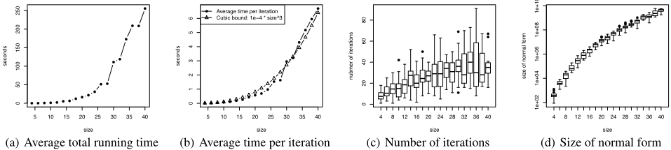
Although Theorem 5 only gives an exponential bound on the number of iterations, the number of iterations in Algorithm 1 grows much more slowly-about linearly-in our experiments, as shown in Figure 1(c). In our experiments, parameters r, b, and d are generated uniformly at random from ¶1↪ ▷ ▷ ▷ ↪ 10♦ (or ¶-10↪ ▷ ▷ ▷ ↪ -1♦). Each instance of size n has n evaders and n sites; for each n we solved 20 instances.
The running time per iteration is provably polynomial and it grows about cubically as Figure 1(b) shows. That is consistent with how the network flow subroutine (which is used in each of our iterations) typically scales.
An alternative approach to solving for these Nash equilibria would be to construct the normal form of the game and use a standard NE-finding algorithm. This approach, however, is doomed regardless of the precise choice of algorithm, because the size of the normal form blows up exponentially, as shown in Figure 1(d).
Note that we implemented our algorithm completely in Python (including the min-cost network flow subroutine). Hence there is room to further improve the performance by using C/C++, and/or some optimized network flow libraries.
7 Future Research
The obvious direction for future research is resolving whether our algorithm in fact provably runs in polynomial time-and, if not, whether there is another algorithm that does. The algorithm's success in experiments gives us hope that the answer to at least one of these two questions is positive, but we have not been able to decisively answer them. There are several indications that the question is inherently difficult to answer. The earlier algorithm for multiple attacker resources in the non-Bayesian case and the proof of the polynomial bound on its runtime [Korzhyk et al., 2011a] were already quite involved, and we showed that the Bayesian case requires us to deal with additional challenging issues (Subsection "Reducing fromMin-Cost Matching"). Still, we believe that the importance of solving Bayesian security games would justify the devotion of further effort to resolving this question, as well as to extending these techniques to related problems.
Acknowledgments
We thank Ronald Parr for his contributions to our early discussions about Bayesian security games. We are also thankful for support from ARO under grants W911NF-12-1-0550 and W911NF-11-1-0332, NSF under awards IIS-0953756, IIS1527434, CCF-1101659, and CCF-1337215, and a Guggenheim Fellowship. Part of this research was done while Conitzer was visiting the Simons Institute for the Theory of Computing.
@inproceedings{ijcai2016p54,
  title     = {Catcher-Evader Games},
  author    = {Li, Yuqian and Conitzer, Vincent and Korzhyk, Dmytro},
  booktitle = {Proceedings of the Twenty-Fifth International Joint Conference on
               Artificial Intelligence, {IJCAI-16}},
  publisher = {AAAI Press / International Joint Conferences on Artificial Intelligence},
  editor    = {Subbarao Kambhampati},
  pages     = {329--336},
  year      = {2016},
  month     = {7},
  url       = {https://ijcai.org/proceedings/2016/54},
}
TY - CPAPER TI - Catcher-Evader Games AU - Li, Yuqian AU - Conitzer, Vincent AU - Korzhyk, Dmytro T2 - Proceedings of the Twenty-Fifth International Joint Conference on Artificial Intelligence, IJCAI-16 PB - AAAI Press / International Joint Conferences on Artificial Intelligence PY - 2016 SP - 329 EP - 336 UR - https://ijcai.org/proceedings/2016/54 ER -Copied
Machine-readable versions of this paper, for tools and AI agents:





