
Security Games with Multiple Attacker Resources
Proceedings of the Twenty-Second International Joint Conference on Artificial Intelligence. Pages 273-278.
https://doi.org/10.5591/978-1-57735-516-8/IJCAI11-056
© 2011 International Joint Conferences on Artificial Intelligence
Abstract
Algorithms for finding game-theoretic solutions are now used in several real-world security applications. This work has generally assumed a Stackelberg model where the defender commits to a mixed strategy first. In general two-player normal-form games, Stackelberg strategies are easier to compute than Nash equilibria, though it has recently been shown that in many security games, Stackelberg strategies are also Nash strategies for the defender. However, the work on security games so far assumes that the attacker attacks only a single target. In this paper, we generalize to the case where the attacker attacks multiple targets simultaneously. Here, Stackelberg and Nash strategies for the defender can be truly different. We provide a polynomial-time algorithm for finding a Nash equilibrium. The algorithm gradually increases the number of defender resources and maintains an equilibrium throughout this process. Moreover, we prove that Nash equilibria in security games with multiple attackers satisfy the interchange property, which resolves the problem of equilibrium selection in such games. On the other hand, we show that Stackelberg strategies are actually NP-hard to compute in this context. Finally, we provide experimental results.
- X. Chen and X. Deng. Settling the complexity of two- player Nash equilibrium. In Proceedings of the An- nual Symposium on Foundations of Computer Science (FOCS), pages 261-272, 2006.
- V. Conitzer and T. Sandholm. Computing the optimal strategy to commit to. In Proceedings of the ACM Con- ference on Electronic Commerce (EC), pages 82-90, Ann Arbor, MI, USA, 2006.
- C. Kiekintveld, M. Jain, J. Tsai, J. Pita, F. Ordóñez, and M. Tambe. Computing optimal randomized re- source allocations for massive security games. In Pro- ceedings of the Eighth International Joint Conference on Autonomous Agents and Multi-Agent Systems (AAMAS), pages 689-696, Budapest, Hungary, 2009.
- D. Korzhyk, V. Conitzer, and R. Parr. Solving Stack- elberg games with uncertain observability. In AAMAS, Taipei, Taiwan, 2011.
- P. Paruchuri, J. P. Pearce, J. Marecki, M. Tambe, F. Ordóñez, and S. Kraus. Playing games for security: An efficient exact algorithm for solving Bayesian Stack- elberg games. In AAMAS, pages 895-902, Estoril, Portu- gal, 2008.
- J. Pita, M. Jain, F. Ordóñez, C. Portway, M. Tambe, and C. Western. Using game theory for Los Angeles airport security. AI Magazine, 30(1):43-57, 2009.
- J. Tsai, S. Rathi, C. Kiekintveld, F. Ordonez, and M. Tambe. IRIS -a tool for strategic security allocation in transportation networks. In AAMAS -Industry Track, pages 37-44, 2009.
- B. von Stengel and S. Zamir. Leadership games with convex strategy sets. Games and Economic Behavior, 69:446-457, 2010.
- Z. Yin, D. Korzhyk, C. Kiekintveld, V. Conitzer, and M. Tambe. Stackelberg vs. Nash in security games: Inter- changeability, equivalence, and uniqueness. In AAMAS, pages 1139-1146, Toronto, Canada, 2010.
References were extracted automatically from the PDF and may contain errors.
Full text extracted automatically from the PDF; figures, tables and equations may differ. The PDF is the version of record.
1 Introduction
Algorithms for computing game-theoretic solutions have recently found several real-world applications to security, including the randomized allocation of checkpoints and canine units at Los Angeles International Airport [5; 6] and of federal air marshals to flights [7]. These security games are generally two-player games between a defender, who allocates defensive resources to targets (or subsets of targets), and an attacker, who chooses which target to attack. The attacked target determines both players' utilities; holding the attacked target fixed, if the target is defended by one of the defender's resources, this increases the defender's utility and decreases the attacker's utility. In spite of their apparently adversarial nature, security games are generally not modeled as zero-sum games.
This leads to a question of which game-theoretic solution concept should be used. One possibility is to solve for a Nash equilibrium of the game. Instead, however, most of the work on these security games assumes that the defender has a Stackelberg leader advantage, where she can commit to a mixed strategy before the attacker moves. One can support the Stackelberg model by arguing that an attacker would spend some time observing the defender's day-to-day actions and thereby learn the defender's mixed strategy before engaging in an attack. The validity of this argument can be debated. Nevertheless, there are advantages to the Stackelberg model, including that being a Stackelberg leader cannot hurt the defender [8], as well as that at least in some cases, such as general two-player normal-form games, computing a Nash equilibrium is PPAD-complete [1] whereas a Stackelberg strategy for the defender can be computed in polynomial time [2].
Security games are a restricted class of games. This additional structure can remove the distinction between Stackelberg and Nash strategies to some extent: if we make certain assumptions about the security game, it turns out that any defender Stackelberg strategy is also a defender Nash strategy [9], though this does not hold in the most general case. The additional structure in security games can also allow for more efficient algorithms. On the other hand, the size of the normal-form representation of the game is generally exponential in the natural parameters of the problem, so that it becomes impractical to apply algorithms based on the normal form.
Kiekintveld et al. [3] define a general class of security games based on allocating defensive resources to targets or subsets of targets. This model was further extended by Yin et al. [9] to allow multiple attacker resources, that is, the attacker can simultaneously attack up to na different targets. This extension is motivated by the fact that terrorist attacks are often performed at multiple locations simultaneously (for example, the 9/11 attacks or the 2008 Mumbai attacks).
In the case of a single attacker resource, Kiekintveld et al. give a simple algorithm called ORIGAMI for the single attacker resource case. It computes a defender strategy that is both a Stackelberg and a Nash strategy (the latter follows from the work of Yin et al. [9]). The main observation used in ORIGAMI is that any Stackelberg strategy for the defender minimizes the attacker's best-response utility. Using this observation, ORIGAMI computes the defender's Nash/Stackelberg strategy by gradually decreasing the attacker's best-response utility, keeping track of the number of defender resources required to bring the attacker's bestresponse utility down to this level, until the number of required defender resources reaches the limit. However, in games with multiple attacker resources, the defender's minimax strategy is not necessarily a Nash or Stackelberg strategy. Consider the following example (from an extended version of Yin et al. [9]). Suppose there are two targets, and the attacker has two resources, so that both targets will be attacked no matter what strategy the defender chooses. If the defender has only one resource, then the defender is better off allocating that resource in such a way that the defender's utility increases the most. However, in the defender's minimax strategy, the defender would allocate the resource so that the attacker's utility is reduced the most. Thus the defender's Nash and Stackelberg strategies can differ from the minimax strategy in this example. In the appendix, we present an example from the extended version of Yin et al. [9] in which the defender's Nash equilibrium strategy differs from the Stackelberg strategy.
In this paper, we give a polynomial-time algorithm for finding a Nash equilibrium in the case of multiple attacker resources. This algorithm can be thought of as a generalization of ORIGAMI in the sense that it also keeps track of the smallest utility that the attacker is going to get from any of his targets, and this utility gradually decreases over the course of the algorithm. However, our algorithm is far more complicated compared to ORIGAMI. Furthermore, we show that Nash equilibria in security games with multiple attacker resources possess the interchange property, which states that as long as each player plays some equilibrium strategy, the resulting strategy profile must be a Nash equilibrium, thus resolving the problem of equilibrium selection for both players. On the other hand, we show that, with multiple attacker resources, computing a defender Stackelberg strategy is actually NP-hard.
2 Security Games, Strategies, and Notation
In the security games that we study, there is a set of targets, T. The defender has nd resources and the attacker has na resources. A pure strategy for the defender (attacker) consists of a subset Sd ⊆ T with |Sd| = nd (Sa ⊆ T with |Sa| = na), corresponding to the targets she defends (he attacks). Targets that are not attacked do not affect either player's utility. Each player's utility is additive over attacked targets. For a target t, the defender receives utility uud (t) if the target is attacked but not defended (uncovered), and ucd (t) if the target is attacked and defended (covered). Similarly, the attacker's utility for an attacked target t is uua (t) in the uncovered case and uca (t) in the covered case. (We require Δud(t) = ucd (t) - uud (t) > 0 and Δua(t) = uua (t) - uca (t) > 0.) Hence, the defender's overall utility is ∑t∈Sa∩Sd ucd (t) + ∑t∈Sa\Sd uud (t), and the attacker's overall utility is ∑t∈Sa∩Sd uca (t)+ ∑t∈Sa\Sd uua (t).
Because of the additive nature of the utility function, the players' expected utilities depend only on the marginal probability that each target is attacked/defended. Hence, a defender mixed strategy can be represented as a vector d = (d1, . . . , d|T|) with ∑t∈T dt = nd, where dt ∈ [0, 1] is the probability that target t obtains a defensive resource, and similarly for the attacker a = (a1, . . . , a|T|) with ∑t∈T at = na, at ∈ [0, 1]. (Note that it does not help to have more than one resource on one target. This assumption was introduced in the security game model by Kiekintveld et al. [3].)
We will use the following shorthand: ua(t, dt) = dtuca (t) + (1 - dt)uua (t) is the attacker's expected utility for attacking target t, and υd(t, at) = atΔud(t) is the marginal expected utility that the defender gets from defending t.
3 Nash Equilibrium
We now consider how to compute a Nash equilibrium, that is, a pair of mixed strategies, one for each player, such that each is a best response to the other. Because of the additive nature of the utility functions, best-responding simply means defending (attacking) the nd (na) targets with the highest utility for the defender (attacker). If there is a tie for the ndth (nath) place, then it is possible to randomize over the corresponding targets. Therefore, d is a best response to a iff there exists some threshold marginal utility θd such that υd(t, at) < θd ⇒ dt = 0 and υd(t, at) > θd ⇒ dt = 1. Similarly, a is a best response to d iff there exists some threshold utility θa such that ua(t, dt) < θa ⇒ at = 0 and ua(t, dt) > θa ⇒ at = 1. Hence, we have a Nash equilibrium iff both these conditions are satisfied. Note that the defender's (and, similarly, the attacker's) strategy can be mixed (randomized), because any target t such that υd(t, at) = θd can be defended with a fractional probability dt ∈ [0, 1]. Similarly, the attacker's strategy can also be mixed.
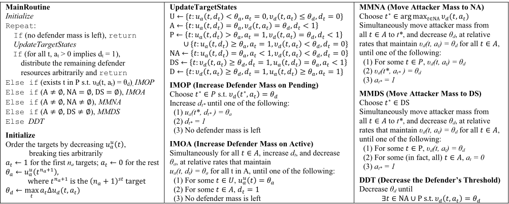
The high-level idea of our algorithm for computing a Nash equilibrium is as follows. We start with a modified game where the defender has no resources at all, for which it is straightforward to compute an equilibrium, and then we gradually increase the number of defender resources (not necessarily to integral amounts), while maintaining an equilibrium of the game as it is changing-until we arrive at the actual number of defender resources. The algorithm transitions among phases that correspond to phases of qualitatively different behavior in the process of increasing the number of defender's resources. The change resulting from a single phase can be computed through a simple calculation.
3.1 Detailed Example Run of the Algorithm
Before we present the algorithm for computing a Nash equilibrium, we first give a detailed example of how it solves a particular game. This example demonstrates the different phases of the algorithm. During these phases, each target will be considered to be in one of 6 possible states: Untouched (U), Newly Attacked (NA), Pending (P), Active (A), Defender Saturated (DS), and Done (D). We will informally introduce every state in this example (precise definitions can be found in the algorithm in Figure 2). The target states depend on the values of the thresholds θa, θd, which are computed at the beginning and gradually decrease during the course of the algorithm.
| t1 [P] | t2[P] | t3[NA] | t4[U] | t1[P] | t2[A] | t3[NA] | t4[U] | t1[P] | t2[A] | t3[A] | t4[U] | t1[P] | t2[A] t3[A] | t4[NA] | ||
|---|---|---|---|---|---|---|---|---|---|---|---|---|---|---|---|---|
| dti | 0 | 0 | 0 | 0 | 0 | 1/3 | 0 | 0 | 0 | 1/3 | 0 | 0 | 0 | 2/3 | 1/3 | 0 |
| ati | 1 | 1 | 0 | 0 | 1 | 1 | 0 | 0 | 1 | 3/5 | 2/5 | 0 | 1 | 3/5 | 2/5 | 0 |
| ua(ti,c) | 5 | 4 | 3 | 2 | 5 | 3 | 3 | 2 | 5 | 3 | 3 | 2 | 5 | 2 | 2 | 2 |
| υd(ti,a) | 1 | 2 | 0 | 0 | 1 | 2 | 0 | 0 | 1 | 6/5 | 6/5 | 0 | 1 | 6/5 | 6/5 | 0 |
(a) Initialize. θd=2, θa=3
(b) IMOP. θd=2, θa=3
(c) MMNA. θd=6/5, θa=3
(d) IMOA. θd=6/5, θa=2
| t1[P] | t2[A] | t3[A] | t4[NA] | t1[A] | t2[A] | t3[A] | t4[NA] | t1[A] | t2[A] | t3[A] | t4[P] | t1[A] | t2[DS] t3[A] | t4[P] | ||
|---|---|---|---|---|---|---|---|---|---|---|---|---|---|---|---|---|
| dti | 0 | 2/3 | 1/3 | 0 | 3/5 | 2/3 | 1/3 | 0 | 3/5 | 2/3 | 1/3 | 0 | 4/5 | 1 | 2/3 | 0 |
| ati | 1 | 1/2 | 1/3 | 1/6 | 1 | 1/2 | 1/3 | 1/6 | 6/11 | 3/11 | 2/11 | 1 | 6/11 | 3/11 | 2/11 | 1 |
| ua(ti,c) | 5 | 2 | 2 | 2 | 2 | 2 | 2 | 2 | 2 | 2 | 2 | 2 | 1 | 1 | 1 | 2 |
| υd(ti,a) | 1 | 1 | 1 | 1/12 | 1 | 1 | 1 | 1/12 | 6/11 | 6/11 | 6/11 | 1/2 | 6/11 | 6/11 | 6/11 | 1/2 |
(e) MMNA. θd=1, θa=2
(f) IMOP. θd=1, θa=2
(g) MMNA. θd=6/11, θa=2
(h) IMOA. θd=6/11, θa=1
| t1[A] | t2[DS] | t3[A] | t4[P] | t1[A] | t2[DS] | t3[A] | t4[A] | t1[A] | t2[D] | t3[A] | t4[A] | t1 | t2 t3 | t4 | ||
|---|---|---|---|---|---|---|---|---|---|---|---|---|---|---|---|---|
| dti | 4/5 | 1 | 2/3 | 0 | 4/5 | 1 | 2/3 | 1/2 | 4/5 | 1 | 2/3 | 1/2 | ≈.806 | 1 | ≈.677 | ≈.516 |
| ati | 1/2 | 1/3 | 1/6 | 1 | 1/2 | 1/3 | 1/6 | 1 | 3/10 | 1 | 1/10 | 3/5 | 3/10 | 1 | 1/10 | 3/5 |
| ua(ti,c) | 1 | 1 | 1 | 2 | 1 | 1 | 1 | 1 | 1 | 1 | 1 | 1 | ≈.968 | 1 | ≈.968 | ≈.968 |
| υd(ti,a) | 1/2 | 2/3 | 1/2 | 1/2 | 1/2 | 2/3 | 1/2 | 1/2 | 3/10 | 2 | 3/10 | 3/10 | 3/10 | 2 | 3/10 | 3/10 |
(i) MMDS. θd=1/2, θa=1
(j) IMOP. θd=1/2, θa=1
(k) MMDS. θd=3/10, θa=1
(l) IMOA. θd=3/10, θa≈.968
Figure 1: The example run of the algorithm. Each subfigure shows the current equilibrium, threshold values, and target states at the end of the corresponding phase.
| t1 | t2 | t3 | t4 | |
|---|---|---|---|---|
| uua | 5 | 4 | 3 | 2 |
| uca | 0 | 1 | 0 | 0 |
| Δud | 1 | 2 | 3 | .5 |
Figure 1 shows the sequence of equilibria for different amounts of defender resources computed by the algorithm. We start with the equilibrium for 0 defender resources. The attacker attacks the two targets that give him the highest utility, namely, t1 and t2 (Fig. 1(a)). Since these two targets are attacked with probability 1, they are likely to get defended as the number of defender resources increases. Thus, these targets are both in the Pending (P) state. Target t4 is in the Untouched (U) state, because ua(t4) < θa, and thus it is neither attacked nor defended.
Increase Defender Mass on Pending (IMOP) phase: We increase the number of defender resources and allocate them to the Pending target t2, which is currently the most appealing to the defender. We cannot put more than 1/3 defender probability on t2 without breaking the attacker's equilibrium condition, so the phase ends at that point. The new equilibrium strategies and updated target states are shown in Figure 1(b).
Move Attacker Mass to Newly Attacked (MMNA) phase: At the beginning of this phase, target t2 is in the Active (A) state, because both players' utilities for defending/attacking this targets are at the corresponding threshold values. Target t3 is in the Newly Attacked (NA) state, because it is currently at the attacker threshold and would start to be attacked if the defender put more probability on t2. In this phase, we move 2/5 of the attacker's probability mass from t2 to t3. As a result, both t2 and t3 now have the highest marginal defender utility (Fig. 1(c)).
Increase Defender Mass on Active (IMOA) phase: We increase the defender probability on Active targets t2 and t3. Since Δua(t2) = Δua(t3), we have to add the same amount of probability to each of these targets; otherwise, the attacker's best-response condition would be broken. We can add up to 1/3 defender probability to these targets, until the attacker's utility for attacking t4 becomes equal to the utility for attacking t2 and t3 (Fig. 1(d)).
MMNA phase: We now move attacker mass from Active targets t2 and t3 to the Newly Attacked t4. To maintain the defender's best-response condition, we need to take mass from t2 and t3 proportionally to 1/Δud(t). We stop when the defender becomes indifferent between t2, t3, and the Pending target t1 (Fig. 1(e)).
IMOP phase: We add 3/5 defender mass to t1, after which the attacker becomes indifferent between all targets (Fig. 1(f)).
MMNA phase: The defender cannot add any mass to her optimal targets t1, t2, and t3, because that would make t4 strictly preferred for the attacker, and the attacker's bestresponse condition would be broken. Therefore, we move attacker mass from t1, t2, t3 to t4 in the right proportions, until the probability on t4 reaches 1 (Fig. 1(g)).
IMOA phase: We can now add defender mass to t1, t2, t3. That will make t4 strictly preferred for the attacker. However, as long as we add mass in the right proportions, the attacker will still be best-responding, because t4 is attacked with probability 1. We stop when the defender probability on t2 becomes 1 and target t2 transitions to the Defender Saturated (DS) phase (Fig. 1(h)).
Move Attacker Mass to Defender Saturated (MMDS) phase: We move attacker mass from t1 and t3 to t2. This does not violate the defender's best-response condition because t2 is already fully defended. We stop when the defender becomes indifferent between t1, t3, and t4 (Fig. 1(i)).
IMOP phase: We increase the defender mass on t4, until the attacker becomes indifferent between all targets (Fig. 1(j)).
MMDS phase: We move attacker mass from Active targets t1, t3, t4 to DS target t2 in the proportions that keep the defender indifferent between the three Active targets, until t2 becomes attacked with probability 1 (Fig. 1(k)).
IMOA phase: We add defender mass to t1, t3, t4, until all defender mass is allocated. After the end of this phase, the algorithm terminates, and the resulting equilibrium profile is an equilibrium of the game with 3 defender resources and 2 attacker resources (Fig. 1(l)).
3.2 Algorithm, Correctness, Runtime
We present the pseudocode for the algorithm in Figure 2. The pseudocode contains the exact definitions of the target states. For proof convenience, we will split the Pending target state into two states: P1 = {t ∈ P : υd(t, at) < θd}, P2 = {t ∈ P : υd(t, at) = θd}.
Theorem 1. Throughout the algorithm, the following holds.
- UpdateTargetStates always assigns each target to exactly one of the states U, A, P1, P2, NA, DS, D.
- At the end of each phase, if the algorithm does not terminate, then at least one target changes its state.
- Each phase terminates.
Proof sketch. It follows from the state definitions that no target can be in two states at the same time. To prove the theorem, we will first show that each target is assigned a state after the initialization phase, and then we will show which targets change states at the end of each phase.
At the beginning of the algorithm, each target is assigned to exactly one state. The na targets for which at = 1 are assigned to the P state, except that targets with at = 1, uua (t) = θa, if any, are assigned to the A state. The other |T| - na targets are assigned to the U state, except that targets with at = 0, uua (t) = θa, if any, are assigned to the NA state.
Next, we specify all target state changes for each phase and for each termination criterion within each phase.
Next, for each phase, we list, for every termination criterion of that phase, which targets change states (always a nonempty set, unless the algorithm terminates). It is straightforward to check that one of these criteria will always apply.
IMOP phase: (1) t∗ becomes A. (2) t∗ becomes D. (3) The algorithm terminates.
IMOA: (1) Every t ∈ U s.t. uua (t) = θa becomes A. (2) Every t ∈ A s.t. dt = 1 becomes either DS (if at < 1) or D (if at = 1). (3) The algorithm terminates.
MMNA: (1) Every t ∈ P s.t. υd(t, at) = θd transitions from P1 to P2. (2) Every t ∈ NA s.t. υd(t, at) = θd becomes A. (3) t∗ transitions fromNA to P1.
MMDS: (1) Every t ∈ P s.t. υd(t, at) = θd transitions from P1 to P2. (2) If this condition happens, then θd = 0, thus at = 0 for all t ∈ P. Also, at = 0 for all t ∈ A, and NA is empty. The algorithm will terminate after this phase because at > 0 implies dt = 1. (3) t∗ transitions to D.
DDT: Every t ∈ NA s.t. υd(t, at) = θd transitions to A. Every t ∈ P s.t. υd(t, at) = θd transitions from P1 to P2.
To complete the proof, we also need to show that no target can change state before the phase is over. This can be done in a straightforward way by carefully checking all state definitions.
Theorem2. Throughout the algorithm, the current strategies 〈d, a〉 constitute a Nash equilibrium for the current number of defender resources.
Proof. This follows immediately from the following facts: (1) each target is always in one of the states (Theorem 1), and (2) each state definition implies that the equilibrium condition with respect to the thresholds (beginning of Section 3) is satisfied for such a state.
Theorem 3. The algorithm terminates after at most 6|T| phases, and each phase requires O(|T |) time.
Proof. We can order the 7 possible states as follows: U < NA < P1 < P2 < A < DS < D. As we can see from the proof of Theorem 1, after each phase (except the last one), some target changes its state to a later state. Thus the algorithm terminates after at most 6|T | phases. In each phase, we can calculate directly at what point the phase will terminate, though this in general requires examining all |T| targets.
3.3 Interchangeability
While we have shown how to compute a Nash equilibrium efficiently, a defender may still be unconvinced about whether she actually wants to play her corresponding strategy. For example, if she has a commitment advantage where the attacker observes her distribution before acting, she would prefer to play a Stackelberg strategy; we will return to this in Section 4. However, even if the attacker cannot observe her distribution, she may worry that she is playing her strategy from the "wrong" equilibrium: in general games, if one player plays according to one equilibrium and the other according to another, the result may be disastrous for both (see the game of chicken). In this section, we alleviate this latter concern, by showing that the security games in this paper satisfy the interchange property: any combination of equilibrium strategies is, in fact, itself an equilibrium. (This was previously shown for a large class of security games with a single attacker resource [9].)
Suppose σ = 〈d, a〉 and σ′ = 〈d′ , a′ 〉 are two NE profiles in a security game with multiple attacker resources. We need to show that 〈d′ , a〉 and 〈d, a′ 〉 are also NE profiles of the same game. We first prove that for any target, either the defender probability on that target is the same in all equilibrium profiles, or the attacker probability is the same in all equilibrium profiles, or both.
Lemma 4. If σ = 〈d, a〉 and σ′ = 〈d′ , a′ 〉 are two NE profiles, then there is no target t for which both (1) the defender probabilities are different in the two profiles and (2) the attacker probabilities are different in the two profiles. In other words, for any target t, at least one of equalities dt = d′t , at = a′t must hold.
Proof. The proof is by contradiction. Suppose that there is a target t for which dt ̸= d′t and at ̸= a′t . We show that the following four cases must all hold even though two are contradictory.
Case "--": There exists a target t1 such that d′t1 < dt1 and a′t1 < at1 . In profile σ, the attacker's utility ua(t1, dt1 ) must be greater than or equal to the threshold value θa, because at1 > 0. Similarly, in profile σ′ , the attacker's utility ua(t1, d′t1 ) must be less than or equal to the threshold θ′a , because a′t1 < 1. At the same time, the attacker's utility for attacking t1 is higher in profile σ′ than in profile σ, because d′t1 < dt1 . Thus, the following three inequalities must hold.
It follows from these three inequalities that θ′a > θa. Because ∑t at = ∑t a′t and a′t1 < at1 , there must exist a target t2 such that a′t2 > at2 . Since a′t2 > 0, it must be the case that ua(t2, d′t2 ) ≥ θ′a . Similarly, because at2 < 1, it must be the case that ua(t2, dt2 ) ≤ θa. Using the last two inequalities and the fact that θ′a > θa, it follows that ua(t2, dt2 ) < ua(t2, d′t2 ), which implies d′t2 < dt2 . By considering the target t2, it follows that the case "-+" must also hold.
Case "-+": There is a target t1 such that d′t1 < dt1 and a′t1 > at1 . The defender's marginal utility for defending target t1 must be at or above the threshold θd in profile σ (because dt1 > 0) and at or below the threshold θ′d in profile σ′ (because d′t1 < 1). At the same time, since t1 is attacked with a higher probability in σ′ than in σ, it must be that υd(t1, a′t1 ) > υd(t1, at1 ). Thus we have θ′d ≥ υd(t1, a′t1 ) > υd(t1, at1 ) ≥ θd. Because ∑t dt = ∑t d′t = nd and d′t1 < dt1 , there must be a target t2 such that d′t2 > dt2 . The defender's marginal utility for defending t2 must be at or above the threshold θ′d in profile σ′ (because d′t2 > 0) and at or below the threshold θd in profile σ (because dt2 < 1). Since
θ′d > θd, it follows that υ(t2, a′t2 ) ≥ θ′d > θd ≥ υ(t2, at2 ), which implies a′t2 > at2 . By considering the target t2, it follows that the case "++" must also hold.
We can also prove the following two implications similarly to the two cases described above, by reversing the roles of equilibria σ and σ′ :
Case "++": There is a target t1 such that d′t1 > dt1 and a′t1 > at1 . If this case holds, then the case "+-" must also hold. This can be proven similarly to the implication "--" ⇒ "-+", by reversing the roles of equilibria σ and σ′ .
Case "+-": There is a target t1 such that d′t1 > dt1 and a′t1 < at1 . If this case holds, then the case "--" must also hold. This can be proven similarly to the implication "-+" ⇒ "++", by reversing the roles of equilibria σ and σ′ .
It follows that if at least one of the cases "--", "-+", "++", "+-" holds, then all of them must hold. But if both "--" and "++" hold, then both inequalities θ′a > θa and θa > θ′a must hold, which is impossible. Hence, none of the four cases can hold.
We now show that in an equilibrium the defender obtains the same marginal utility from all targets that have different defender probabilities in a different equilibrium.
Lemma 5. Suppose that σ and σ′ are two NE profiles, and t1, t2 are two targets such that dt1 ̸= d′t1 and dt2 ̸= d′t2 . Then υd(t1, at1 ) = υd(t2, at2 ) = υd(t1, a′t1 ) = υd(t2, a′t2 ).
Proof. Because ∑t dt = ∑t d′t = nd, it is enough to show that υd(t1, at1 ) = υd(t2, at2 ) holds for any pair of targets t1, t2 such that dt1 < d′t1 and dt2 > d′t2 . (This is because if (say) dt1 < d′t1 and dt2 < d′t2 , there must exist a third target t3 with dt3 > d′t3 , so that we can then conclude υd(t1, at1 ) = υd(t3, at3 ) = υd(t2, at2 ).)
In profile σ, the defender can shift her probability from t2 to t1, because dt2 > 0 and dt1 < 1. Since σ is an equilibrium profile, the defender must not benefit from such a shift of probability. Thus υd(t1, at1 ) ≤ υd(t2, at2 ). Using a similar argument for profile σ′ , we get υd(t1, a′t1 ) ≥ υd(t2, a′t2 ). It also follows from Lemma 4 that at1 = a′t1 and at2 = a′t2 . Hence, we have υd(t1, at1 ) ≤ υd(t2, at2 ) = υd(t2, a′t2 ) ≤ υd(t1, a′t1 ) = υd(t1, at1 ), so it follows that these four quantities are all the same.
In the following lemma, we show that any defender's NE strategy is a best-response to any attacker's NE strategy.
Lemma 6. If σ = 〈d, a〉 and σ′ = 〈d′ , a′ 〉 are two NE profiles, then d′ is a best-response to a.
Proof. We will show that the defender's utility for playing strategy d′ against a is the same as the defender's utility for playing d against a. First, note that ud(d′ , a) - ud(d, a) = ∑t:d′t ̸=dt [d′t - dt] υd(t, at). Consider any target t∗ such that dt∗ ̸= d′t∗. Using Lemma 5, we can rewrite the difference in the utilities as follows: ud(d′ , a) - ud(d, a) = υd(t1, at1 ) ∑t:d′t ̸=dt [d′t -dt] = 0. The last summation is equal to zero because ∑t dt = ∑t d′t .
The following lemma can be proven similarly to Lemma 6, by switching from the defender's to the attacker's perspective.
Lemma 7. If σ = 〈d, a〉 and σ′ = 〈d′ , a′ 〉 are two NE profiles, then a′ is a best-response to d.
The interchange property follows from Lemmas 6 and 7.
Theorem 8. If σ = 〈d, a〉 and σ′ = 〈d′ , a′ 〉 are two NE profiles in a security game with multiple attacker resources, then 〈d′ , a〉 and 〈d, a′ 〉 are also NE profiles in that game.
3.4 Experimental Results
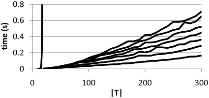
We now show experimental results for our implementation of the algorithm (Figure 3). For given |T |, nd, na, we randomly draw uua and ucd from {1, . . . , 100}, and then we randomly draw uca from {0, . . . , uua - 1} and uud from {0, . . . , ucd - 1}. Each data point averages over 20 games. As a sanity check, our implementation verified that the strategies computed for each game did constitute a Nash equilibrium. The quadratic runtime of the algorithm is reflected in the experimental results. We note that the numbers of pure strategies for the players are (|T| nd ) and (|T| na ), so any alternative algorithm that is based on writing out the normal form is doomed to exponential space (and hence, time) requirements. The time to compute the (|T| nd ) × (|T | na ) utility matrix of the normal-form game for nd = na = 10 is shown in Figure 3 with a dashed line. We can see that our algorithm scales well in the number of targets and attacker resources.
4 NP-Hardness of Computing Stackelberg Strategies
We now turn to the problem of computing a defender Stackelberg strategy. d is an optimal mixed strategy to commit to or Stackelberg strategy for the defender if there exists some a that is a best response to d such that for any alternative strategies 〈d′ , a′ 〉, where a′ is a best response to d′ , we have ud(d, a) ≥ ud(d′ , a′ ).
Theorem 9. In security games with multiple attacker resources, finding an optimal defender Stackelberg strategy is weakly NP-hard. This holds even when the defender has only one resource, and the defender's utility for a target does not depend on whether she has a resource there (that is, ucd (t) = uud (t) for all t). 12
Proof sketch. We reduce an arbitrary knapsack problem instance-given by k items, where each item j is defined by a pair (wj, vj), and we are asked if there is a subset S of the items with ∑j∈S wj ≤ 1 and ∑j∈S vj ≥ V -to the following game. We construct a game with 2k targets, in which the defender has one resource and the attacker has k resources. Targets t1, . . . , tk correspond to the items in the knapsack, and the utilities are set up as follows for 1 ≤ i ≤ k.
Targets tk+1, . . . , t2k are "dummy" targets, so that for k+1 ≤ i ≤ 2k: uua (ti) = uca (ti) = ucd (ti) = uud (ti) = 0.
Let the vector d represent the defender's strategy, so that di is the probability of target ti being covered. If dti ≥ wi for 1 ≤ i ≤ k, the attacker attacks a dummy target instead of ti, thus increasing the defender's utility by vi.
There exists attacker's pure-strategy best-response to the defender's Stackelberg strategy (with ties broken in the defender's favor) such that the optimal subset S of the items in the knapsack corresponds to the targets ti with 1 ≤ i ≤ k and ati = 0. It can be shown that the defender can get a utility of at least V - ∑ki=1 vi if and only if the knapsack instance has a solution (with value at least V ).
5 Future Research
Future research can take a number of directions. Can the algorithm that we presented in this paper be generalized to richer settings? For example, is it possible to compute Nash equilibria efficiently in cases where either defender resources or attacker resources (or both) are heterogeneous? (With heterogeneous resources, not every resource can defend/attack every target. Our work in this paper assumes homogeneous resources.) Can we efficiently compute them in (restricted) settings with schedules? (A schedule is a subset of targets that can be simultaneously defended/attacked by a single resource.)
1 We have also found a pseudopolynomial-time algorithm (not presented here) for the special case where ucd(t) = uud(t) for all t.
2 Note that this violates the assumption that ucd(t) > uud(t). It is easy to modify the utilities by ϵ so that this property holds again and the reduction still works.
In the extended version of the paper by Yin et al. [9], a model with uncertainty about whether the attacker can observe the defender's commitment has been proposed; setting this probability of observability to 0 corresponds to the Nash case, whereas setting it to 1 corresponds to the Stackelberg case. In follow-up work [4], we have designed an algorithm that computes a solution for this richer game model, using Nash and Stackelberg solvers as subroutines. For the case of multiple attacker resources, the algorithm for computing a Nash equilibrium that we have given in this paper can be used as the Nash subroutine; in future research, perhaps an algorithm to compute a Stackelberg strategy can be given that, in spite of the NP-hardness of the problem proven here, nevertheless runs fast in practice.
Beyond security games, it is interesting to investigate further the relationship between Stackelberg strategies and Nash equilibrium strategies, especially regarding whether they can be efficiently computed. We now know of settings where Stackelberg strategies are easier to compute (general twoplayer normal-form games) as well as settings where Nash equilibria are easier to compute (this paper). Is there a general principle that informs us when each one is easy to compute?
6 Acknowledgements
We would like to acknowledge NSF IIS-0812113, CAREER0953756, ARO 56698-CI, and an Alfred P. Sloan Research Fellowship for support. Any opinions, findings, and conclusions or recommendations in this document are those of the authors and do not necessarily reflect views of the funding agencies. We also thank the anonymous reviewers for valuable suggestions.
A An Example inWhich the Defender's Nash Equilibrium Strategy is Different from the Stackelberg Strategy
Consider the following example game (from the extended version of Yin et al. [9]) in which the defender's Nash equilibrium strategy is different from the defender's Stackelberg (SSE) strategy. In this example, the defender has one resource, the attacker has two resources, and the utilities are set up as shown in the following table.
| t1 | t2 | t3 | ||||
|---|---|---|---|---|---|---|
| Def | Cov. 0 | Uncov. -2 | Cov. -9 | Uncov. -10 | Cov. 0 | Uncov. -1 |
| Att | 5 | 6 | 2 | 4 | 1 | 3 |
In this game, the defender has a unique Nash equilibrium strategy and a unique Stackelberg strategy, which can be computed as follows (quoting the extended version of Yin et al. [9]):
t1 must be attacked with probability 1. Because Δud(t1) = 2 > 1 = Δud(t2) = Δud(t3), in NE, this implies that the defender must put her full probability 1 on t1. Hence, the attacker will attack t2 with his other resource. So, the unique NE profile is 〈(1, 0, 0), (1, 1, 0)〉.
In contrast, in SSE, the defender's primary goal is to avoid an attack on t2, which requires putting probability at least .5 on t2 (so that the attacker prefers t3 over t2). This will result in t1 and t3 being attacked; the defender prefers to defend t1 with her remaining probability because Δud(t1) = 2 > 1 = Δud(t3). Hence, the unique SSE profile is 〈(.5, .5, 0), (1, 0, 1)〉.
@inproceedings{ijcai2011p56,
  title     = {Security Games with Multiple Attacker Resources},
  author    = {Korzhyk, Dmytro and Conitzer, Vincent and Parr, Ronald},
  booktitle = {Proceedings of the Twenty-Second International Joint Conference on
               Artificial Intelligence, {IJCAI-11}},
  publisher = {AAAI Press/International Joint Conferences on Artificial Intelligence},
  editor    = {Toby Walsh},
  pages     = {273--278},
  year      = {2011},
  month     = {7},
  doi       = {10.5591/978-1-57735-516-8/IJCAI11-056},
  url       = {https://doi.org/10.5591/978-1-57735-516-8/IJCAI11-056},
}
TY - CPAPER TI - Security Games with Multiple Attacker Resources AU - Korzhyk, Dmytro AU - Conitzer, Vincent AU - Parr, Ronald T2 - Proceedings of the Twenty-Second International Joint Conference on Artificial Intelligence, IJCAI-11 PB - AAAI Press/International Joint Conferences on Artificial Intelligence PY - 2011 SP - 273 EP - 278 DO - 10.5591/978-1-57735-516-8/IJCAI11-056 UR - https://doi.org/10.5591/978-1-57735-516-8/IJCAI11-056 ER -Copied
Machine-readable versions of this paper, for tools and AI agents:





