
Game-Theoretic Question Selection for Tests
Proceedings of the Twenty-Third International Joint Conference on Artificial Intelligence. Pages 254-261.
© 2013 International Joint Conferences on Artificial Intelligence
Abstract
Conventionally, the questions on a test are assumed to be kept secret from test takers until the test. However, for tests that are taken on a large scale, particularly asynchronously, this is very hard to achieve. For example, example TOEFL iBT and driver's license test questions are easily found online. This also appears likely to become an issue for Massive Open Online Courses (MOOCs). In this paper, we take the loss of confidentiality as a fact. Even so, not all hope is lost as the test taker can memorize only a limited set of questions' answers, and the tester can randomize which questions appear on the test. We model this as a Stackelberg game, where the tester commits to a mixed strategy and the follower responds. We provide an exponential-size linear program formulation, prove several NP-hardness results, and give efficient algorithms for special cases.
- [Birkhoff, 1946] Garrett Birkhoff. Tres observaciones sobre el algebra lineal. Univ. Nac. Tucumn Rev, Ser. A, no. 5, pages 147-151, 1946.
- [Chang et al., 2001] Cheng-Shang Chang, Wen-Jyh Chen, and Hsiang-Yi Huang. Coherent cooperation among com- municating problem solvers. IEEE Transactions on Com- munications, 49(7):1145-1147, July 2001.
- [Chen et al., 2009] Xi Chen, Xiaotie Deng, and Shang-Hua Teng. Settling the complexity of computing two-player Nash equilibria. Journal of the ACM, 56(3), 2009.
- [Conitzer and Sandholm, 2006] Vincent Conitzer and Tuo- mas Sandholm. Computing the optimal strategy to commit to. In ACM EC, pages 82-90, Ann Arbor, MI, USA, 2006.
- [Conitzer and Sandholm, 2008] Vincent Conitzer and Tuo- mas Sandholm. New complexity results about Nash equi- libria. Games and Economic Behavior, 63(2):621-641, 2008.
- [Cooper and Sahami, 2013] Steve Cooper and Mehran Sa- hami. Reflections on Stanford's MOOCs. Communica- tions of the ACM, 56(2):28-30, February 2013.
- [Daskalakis et al., 2009] Constantinos Daskalakis, Paul Goldberg, and Christos H. Papadimitriou. The complexity of computing a Nash equilibrium. SIAM Journal on Computing, 39(1):195-259, 2009.
- [Dulmage and Halperin, 1955] Lloyd Dulmage and Israel Halperin. On a theorem of Frobenius-Konig and J. von Neumann's game of hide and seek. Trans. Roy. Soc. Canada III, 49:23-29, 1955.
- [Edmonds and Karp, 1972] Jack Edmonds and Richard M. Karp. Theoretical improvements in algorithmic effi- ciency for network flow problems. Journal of the ACM, 19(2):248-264, 1972.
- [Gilboa and Zemel, 1989] Itzhak Gilboa and Eitan Zemel. Nash and correlated equilibria: Some complexity consid- erations. Games and Economic Behavior, 1:80-93, 1989.
- [Goldberg and Tarjan, 1988] Andrew V. Goldberg and Robert E. Tarjan. A new approach to the maximum-flow problem. Journal of the ACM, 35(4):921-940, 1988.
- [Han, 1997] C.-C. Han. A fast algorithm for the minimax flow problem with 01 weights. Applied Mathematics Let- ters, 10(1):11 -16, 1997.
- [Jain et al., 2008] Manish Jain, James Pita, Milind Tambe, Fernando Ordóñez, Praveen Paruchuri, and Sarit Kraus. Bayesian Stackelberg games and their application for se- curity at Los Angeles International Airport. SIGecom Exch., 7(2):1-3, 2008.
- [Jain et al., 2011] Manish Jain, Christopher Kiekintveld, and Milind Tambe. Quality-bounded solutions for finite Bayesian Stackelberg games: Scaling up. In AAMAS, pages 997-1004, Taipei, Taiwan, 2011.
- [Khachiyan, 1979] Leonid Khachiyan. A polynomial al- gorithm in linear programming. Soviet Math. Doklady, 20:191-194, 1979.
- [Kiekintveld et al., 2009] Christopher Kiekintveld, Manish Jain, Jason Tsai, James Pita, Fernando Ordóñez, and Milind Tambe. Computing optimal randomized resource allocations for massive security games. In AAMAS, pages 689-696, Budapest, Hungary, 2009.
- [Korzhyk et al., 2010] Dmytro Korzhyk, Vincent Conitzer, and Ronald Parr. Complexity of computing optimal Stack- elberg strategies in security resource allocation games. In AAAI, pages 805-810, Atlanta, GA, USA, 2010.
- [Korzhyk et al., 2011] Dmytro Korzhyk, Zhengyu Yin, Christopher Kiekintveld, Vincent Conitzer, and Milind Tambe. Stackelberg vs. Nash in security games: An extended investigation of interchangeability, equiva- lence, and uniqueness. Journal of Artificial Intelligence Research, 41(2):297-327, 2011.
- [Letchford and Conitzer, 2013] Joshua Letchford and Vin- cent Conitzer. Solving security games on graphs via marginal probabilities. 2013.
- [Letchford et al., 2009] Joshua Letchford, Vincent Conitzer, and Kamesh Munagala. Learning and approximating the optimal strategy to commit to. In Proceedings of the Sec- ond Symposium on Algorithmic Game Theory (SAGT-09), pages 250-262, Paphos, Cyprus, 2009.
- [Paruchuri et al., 2008] Praveen Paruchuri, Jonathan P. Pearce, Janusz Marecki, Milind Tambe, Fernando Ordóñez, and Sarit Kraus. Playing games for security: An efficient exact algorithm for solving Bayesian Stackelberg games. In AAMAS, pages 895-902, Estoril, Portugal, 2008.
- [Pita et al., 2009] James Pita, Manish Jain, Fernando Ordóñez, Christopher Portway, Milind Tambe, and Craig Western. Using game theory for Los Angeles airport security. AI Magazine, 30(1):43-57, 2009.
- [Shieh et al., 2012] Eric Shieh, Bo An, Rong Yang, Milind Tambe, Craig Baldwin, Joseph DiRenzo, Ben Maule, and Garrett Meyer. PROTECT: A deployed game theoretic system to protect the ports of the United States. In AA- MAS, Valencia, Spain, 2012.
- [Tsai et al., 2009] Jason Tsai, Shyamsunder Rathi, Christo- pher Kiekintveld, Fernando Ordonez, and Milind Tambe. IRIS -a tool for strategic security allocation in transporta- tion networks. In AAMAS, pages 37-44, Budapest, Hun- gary, 2009.
- [von Neumann, 1928] John von Neumann. Zur Theorie der Gesellschaftsspiele. Mathematische Annalen, 100:295- 320, 1928.
- [von Stengel and Zamir, 2010] Bernhard von Stengel and Shmuel Zamir. Leadership games with convex strategy sets. Games and Economic Behavior, 69:446-457, 2010.
- [Yin et al., 2012] Zhengyu Yin, A Jiang, M Johnson, Milind Tambe, Christopher Kiekintveld, Kevin Leyton-Brown, Tuomas Sandholm, and John Sullivan. Trusts: Scheduling randomized patrols for fare inspection in transit systems. In Proc. of the 24th Conference on Innovative Applications of Artificial Intelligence, IAAI, 2012.
References were extracted automatically from the PDF and may contain errors.
Full text extracted automatically from the PDF; figures, tables and equations may differ. The PDF is the version of record.
1 Introduction
Massive Open Online Courses (MOOCs) have emerged quite spectacularly and there is much speculation about how their role in society will develop (for a recent discussion, see [Cooper and Sahami, 2013]). In particular, the issue of how the students' accomplishments can be efficiently validated and certified is often discussed. One approach that is now used is to allow students to take a proctored exam in a testing center. A potential vulnerability of this approach is that the questions used on a test may be leaked, online or otherwise. Certainly, this is already the case for other tests that are taken asynchronously by many people, such as the TOEFL iBT and driver's license tests. A similar issue occurs for interview questions, particularly those with a "puzzle" flavor. A natural approach to addressing this is to generate enough questions that a test taker would be unable to memorize them all, and then to select from these questions randomly on each instantiation of the test.
However, sampling test questions uniformly at random may be suboptimal for several reasons. Some questions may be more effective than others at identifying test takers that do not know the material; should these be used more often?
Also, it may be not be optimal to consider questions in isolation; it is likely better to use two questions that test very different parts of the material than ones that are quite similar. At the same time, choosing the test questions deterministically is obviously fatally flawed, as this makes it easy to memorize the questions. Instead, a more intelligent form of randomization seems desired. Game theory provides a natural framework to determine such a randomized strategy. We can model the test as a game between the tester, who chooses questions for the test, and the test taker, who chooses for which questions (on material that he has not mastered) to memorize the answers. This is the approach that we take in this paper.
We model the test game as a Bayesian game, in which there is uncertainty about the type of the test taker. We assume here the availability of detailed statistical data on the different types of test takers, specifically concerning their mastery of various material that is potentially on the test, and their ability to memorize answers. Our primary focus is on the computational problem of, given this data, determining an optimal mixed strategy for the tester to determine what is on the test.
While we have used exams and similar tests as motivating examples in the above, there are other potential applications in which some entity is being examined in a limited way. For example, a team of (say, nuclear) inspectors may be able to visit only a limited number of suspect sites (corresponding to being able to place only a limited number of questions on an exam). The entity being investigated may be able to cover up illicit activity at a limited number of sites (corresponding to memorizing the answers to selected questions), and many of the sites may not have any illicit activity in the first place (corresponding to questions that the test taker can handle without having to memorize the answer).
Related Work. The computation of Stackelberg mixed strategies has recently been applied to a number of real security domains [Pita et al., 2009; Tsai et al., 2009; Shieh et al., 2012; Yin et al., 2012]. The main reason for using a Stackelberg formulation in these domains is that in many of them, an attacker could observe the defender's actions over time and thereby learn the defender's strategy before acting; the same can be argued for the domain that we are studying here. The Stackelberg model also largely avoids the possible equilibrium selection problems of a simultaneous-move model. Another advantage is that a Stackelberg strategy of a two-player normal-form game can be computed in polynomial time [Conitzer and Sandholm, 2006; von Stengel and Zamir, 2010], whereas computing one Nash equilibrium is PPAD-complete [Daskalakis et al., 2009; Chen et al., 2009] and computing an (even approximately) optimal Nash equilibrium is NP-hard [Gilboa and Zemel, 1989; Conitzer and Sandholm, 2008]. However, for Bayesian games (which we study here), computing an optimal (or even approximately optimal) Stackelberg strategy is NP-hard [Conitzer and Sandholm, 2006; Letchford et al., 2009]. Mixed integer program and heuristic branch-and-bound approaches have been used to tackle this problem and have turned out to be reasonably scalable [Jain et al., 2008; 2011]. Our approach is very different. We modify the Bayesian Stackelberg game into a Bayesian zero-sum game by exploiting our problem's structure, allowing us to use a much more efficient minimax LP.
Of course, problem structure has also been exploited in previous work on security games. Kiekintveld et al. proposed a quite general (though not all-encompassing) model of security games [Kiekintveld et al., 2009]. In it, the defender assigns resources to targets (or sets of targets), and the attacker chooses a single target to attack. The size of the normal form of these games is exponential in the natural representation size, but a more compact MIP/LP formulation can be given whose size is polynomial [Kiekintveld et al., 2009]. However, this formulation is correct only under certain conditions (for example, each resource can be assigned only to a single target), and when these do not hold NP-hardness is usually encountered [Korzhyk et al., 2010; Letchford and Conitzer, 2013]. Similarly, in this paper, we give a polynomial-size LP for the case where only a single question is tested, but show NP-hardness results for more general settings. (Our general minimax LP has exponential size in the natural representation of the problem.)
It has also been shown that under mild conditions, in security games, Stackelberg strategies are guaranteed to also be Nash and minimax strategies [Korzhyk et al., 2011], though this is not true in Bayesian versions of security games. In general, while there are some high-level similarities between our results and previous results on security games, we do not know how to draw a formal connection. In some ways, the role of the tester seems analogous to that of the attacker (with the test-taker "defending" certain questions by studying them); on the other hand, the tester is the natural Stackelberg leader and in that sense resembles the defender in security games. In the appendix, we show that if we do make the test taker the Stackelberg leader, the zero-sum equivalence that we demonstrate and rely on no longer holds.
2 Definitions and Notation
A test game G = (Q, Θ, p, t, u1, u2) is a 2-player Bayesian game between the tester (player 1) and the test taker (player 2). The tester has a set of potential test questions Q = {q1, q2, . . . , qn}. 1 The test taker has a type θ ∈ Θ (|Θ| = L) that characterizes which questions are hard for the test taker (i.e., which questions he would not be able to answer without memorizing them), and howmany questions the test taker can memorize. That is, θ = (Hθ,mθ), where Hθ ⊆ Q is the set of questions that are hard for θ, and mθ ∈ N is the number of questions for which θ would be able to memorize the answer, so that a test taker of type θ has (|Hθ| mθ ) pure courses of action. (W.l.o.g., mθ ≤ |Hθ|.) p : Θ → [0, 1] is the probability distribution over types. The tester can put t questions on the test, and thus has (nt ) pure strategies. We use T to denote such a pure strategy, andMθ to denote the subset of questions that θ memorizes. u1(θ, T,Mθ) denotes the tester's utility for type θ, and u2(θ, T,Mθ) denotes the utility of a type θ test taker.
1 In common parlance, "problem" may be a better word, but this runs the risk of confusion with our computational problems.
In general, the utility functions could be very rich, depending in a complicated way on the true type and the number (or even precise set) of questions answered correctly. To avoid getting too deeply into the modeling aspects of this, we study only a case that should be a special case of most reasonable models. This strengthens the hardness results that we obtain later in the paper (since these hardness results automatically also apply to the richer models of which our model is a special case), though it weakens our positive results. Specifically, we assume that the only two outcomes of the test are to pass or fail the test taker. Moreover, we assume that the tester does not want to pass any test taker that cannot answer all the questions (without memorizing any). Thus, the tester will pass exactly the agents that answer all the questions on the test correctly. Agents that can answer all the questions without memorizing any have no strategic decisions to make and will always pass; therefore, we do not model them explicitly as a type in the game. (They can be thought of as adding a constant to the tester's utility function that is sufficiently large that the tester indeed wants to pass agents that answer all questions correctly.)
Thus, for the explicitly modeled types θ (which the tester wants to fail), we assume that u1(θ, T,Mθ) = 0 if T ∩ (Hθ \Mθ) ̸= ∅ (i.e., a question is tested that the agent cannot answer, so the the agent fails) and u1(θ, T,Mθ) = -vθ otherwise (the cost of passing an agent of type θ). For the test takers, u2(θ, T,Mθ) = 0 if T ∩ (Hθ \ Mθ) ̸= ∅, and u2(θ, T,Mθ) = ωθ otherwise. We require vθ, ωθ > 0.
We believe that a Stackelberg model is most natural for our setting, where the tester first commits to a mixed strategy, and the test takers observe this mixed strategy and bestrespond. This is because the test takers can observe and learn the tester's strategy over time. Arguably, however, if the test takers are not able to do such learning, a Nash equilibrium model (i.e., no Stackelberg leadership) also makes sense. In the next section, we show that in fact, both of these models are equivalent to the same zero-sum game.
3 Equivalence to a Zero-SumGame
For any test game G as defined above, we can modify it into a zero-sum game G′ by substituting the following utility function for the test taker: u′2 (θ, T,Mθ) = 0 if T∩(Hθ\Mθ) ̸= ∅, and u′2 (θ, T,Mθ) = vθ otherwise.
Proposition 1. The set of Stackelberg mixed strategies for the tester in G is equal to the set of maximin strategies for the tester in G′ . These sets are also equal to the set of Nash equilibrium strategies for the tester in G.
Proof. First, we argue that the sets of Stackelberg mixed strategies for the tester in G and G′ are the same. This follows from the fact that every test taker type simply acts to maximize his probability of passing, whether the utility function is u2 or u′2 . Second, it is well known that in a 2-player zero-sum game, the set of Stackelberg mixed strategies is equal to the set of maximin strategies for the leader.
Similarly, the sets of Nash equilibrium strategies for the tester in G and G′ are the same. This again follows from the fact that every test taker type simply acts to maximize his probability of passing, for either utility function. Finally, in a 2-player zero-sum game, the set of Nash equilibrium strategies is equal to the set of maximin strategies for the leader (by the minimax theorem [von Neumann, 1928]).
We note that the equivalence to this zero-sum game is not complete, in the sense that it would not hold if the test taker is a Stackelberg leader who can commit to a strategy (before learning his type). An example is provided in Appendix A. However, since this reversed Stackelberg model is not of primary interest to us, we proceed with the zero-sum formulation from here on, focusing on G′ knowing that its solution will give us a solution to our original problem.
4 General Linear Program (LP) Formulation
Computing an optimal Stackelberg mixed strategy in a general 2-player Bayesian game is NP-hard [Conitzer and Sandholm, 2006] and inapproximable [Letchford et al., 2009]; a general mixed-integer linear program formulation has previously been proposed [Paruchuri et al., 2008]. However, thanks to Proposition 1, we only need to solve for a maximin strategy of a zero-sum game. The following linear programming approach is standard:
Here, Vθ is the utility that the tester receives from type θ, and xT is the probability of testing exactly the questions in T.
The dual of the above LP is:
The variables of the dual LP yθ,Mθ give a strategy for the test taker that maps types to probabilities of memorizing subsets of questions: the probability of memorizing Mθ conditional on having type θ is yθ,Mθ /p(θ). U = maxT⊆Q:|T|=t UT is the best-response utility for the tester, where UT = ∑θ,Mθ⊆Hθ:|Mθ|=mθ u1(θ, T,Mθ)yθ,Mθ is the utility of testing T. By linear programming duality, the two LPs have the same optimal solution value (corresponding to the minimax theorem); strategies corresponding to optimal solutions of these LPs constitute an equilibrium of the game.
Linear programs can be solved in time polynomial in their size [Khachiyan, 1979]. However, while the size of the LPs above is polynomial in the size of the game matrix, it is nevertheless exponential in the size of the natural representation of our test games. The tester's pure strategy space is exponential in t (the number of questions to test) and space of pure courses of action for a test taker of type θ is exponential in mθ (the number of questions whose answers he can memorize). When t and maxθ mθ are constant, the LPs indeed give us a polynomial-time algorithm. But, can the test game be solved in polynomial time when either the number of questions to test, the number of answers to memorize, or both are not constant?
5 Constant Memory Size
In this section, we study the case where memory size (maxθ mθ) is constant, but test size t is not. We first define a decision variant of our problem:
Definition 1 (The OPTIMAL TEST STRATEGY problem). Given a test game G and a value u, the OPTIMAL TEST STRATEGY problem is to decide whether the tester has a strategy that gives her a utility of at least u (when the test taker best-responds).
Proposition 2. When memory size (maxθ mθ) is constant, OPTIMAL TEST STRATEGY is in NP.
Proof. When maxθ mθ is constant, the number of constraints (not counting the nonnegativity constraints on the variables) in LP (1) is polynomial. Any LP has an optimal solution with a number of nonzero variables that is at most the number of constraints (not counting the nonnegativity constraints)-this follows, for example, from the simplex algorithm. Hence, a subset of the variables of this LP of this size can serve as a certificate: we can solve the LP restricted to these variables in polynomial time, and check whether the optimal solution is at least u.
We now prove that the problem is in fact NP-hard, even when the test taker cannot memorize any questions!
Theorem 1. Even if the test taker cannot memorize any questions (mθ = 0) and |Hθ| = 2 for all θ ∈ Θ, OPTIMAL TEST STRATEGY is NP-hard.
Proof. We reduce from the VERTEX COVER problem, in which we are given a graph (V,E) and a number k, and are asked whether there exists a subset of k vertices such that every edge is incident on at least one of these vertices. For any instance of this problem, we construct an OPTIMAL TEST
STRATEGY instance as follows. Let Q = V . For each edge e = {i, j} ∈ E, add one type of test taker θe whose hard question set Hθe = e. Let p(θe) = 1/|E|, vθe = 1 and mθe = 0 for all e ∈ E. Finally, let t = k and u = 0.
If there exists a vertex cover, consider the tester strategy of testing exactly these questions. Then, every type will fail at least one question and hence the test, resulting in a utility of 0 for the tester.
Conversely, if there exists a tester strategy that gives the tester a utility of 0, then every type passes the test with probability 0 under this tester strategy. Thus, consider any T ⊆ Q with |T| = k that gets positive probability; every type must fail this test. This means that T includes at least one endpoint of every edge, i.e., it is a vertex cover.
6 Constant Test Size
In this section, we study the case where test size is constant, but memory size is not.
Proposition 3. When the test size (t) is constant, OPTIMAL TEST STRATEGY is in coNP.
Proof. When t is constant, the number of constraints (not counting the nonnegativity constraints on the variables) in LP (2) is polynomial. As in the proof of Proposition 2, this implies that a subset of the variables of this LP of the requisite size can serve as a certificate that u cannot be achieved: we can solve the LP restricted to these variables in polynomial time, and check whether the optimal solution is strictly less than u. If so, then by weak duality, it is impossible for the tester to obtain u or more (and moreover, by strong duality, if it is not possible for the tester to obtain u or more, such a certificate must exist).
Theorem 2. Even if the test size t is 2 and there are only two types that can memorize any answers, OPTIMAL TEST STRATEGY is coNP-hard.
Sketch of Proof. In the full version of this paper, we reduce from the INDEPENDENT SET problem, in which we are given a graph (V,E) and a number k, and are asked whether there exists a subset of k vertices such that no two of these vertices have an edge between them. For any instance of this problem, we construct an OPTIMAL TEST STRATEGY instance that has a "no" answer if and only if the INDEPENDENT SET instance has a "yes" answer. The vertices correspond to questions. We create several types that cannot memorize anything; these ensure that the tester is best off testing exactly the pairs of questions that are not edges. Then, we create two more types for which all questions are hard and that can memorize k answers and 2 answers, respectively. The tester will be worst off if the former type memorizes an independent set (thereby covering (k2) non-edge pairs of questions) and the latter spreads his mass equally across all the other non-edge pairs. □
7 Tests of Size One
Theorem 1 shows that when we do not bound the test size, our problem is hard even if test takers cannot memorize anything. But, if we do not bound the memory size, Theorem 2
only shows that our problem is hard if the tester can test two questions simultaneously. This still leaves open whether an efficient algorithm exists when the test size is restricted to 1. In this section, we show that this is in fact the case. Our interest in this special case derives not only from it being left open by our hardness results, but also from potentially important applications. For one, an interviewer often only has time to ask an applicant a single question. Moving away from interpreting questions literally, a (for example) nuclear inspections team may be able only to inspect a single site (within a particular time frame).
In this special case, LP (1) has polynomially many variables, but an exponential number of constraints. A quick proof of the polynomial-time solvability of this case is given by establishing that there is a polynomial-time separation oracle for finding a violated constraint. This separation oracle is straightforward: simply select, for every type θ, the mθ questions in Hθ that get the highest probability xq in the current solution (breaking ties arbitrarily), and see whether the corresponding constraint is violated. However, in this section, we develop more direct approaches that do not require generating violated constraints and that give more insight into the structure of the solution.
7.1 Linear Program
We first present a linear program that can be thought of as a polynomial-size version of LP (2). Instead of variables yθ,Mθ , this linear program has a variable zθ,q for every individual q ∈ Hθ. These variables correspond to the marginal probability that θ memorizes q (in this case, conditional on θ being the type). In the case where the tester tests one question, these marginal probabilities are all that matter. (This is not true when the tester tests more than one question, because in that case, for example, if the tester always tests two questions together, a test taker may be best off memorizing the answers either to both questions or to neither question.) Let U 0 q be the utility that the tester obtains when she tests q and nobody memorizes q, i.e., U 0 a = ∑θ:q/∈Hθ p(θ)(-vθ).
Solving LP (3) gives us an equilibrium test taker strategy. 2
2 To be precise, we have to find a test taker strategy that has these marginal probabilities. This is quite straightforward in this context: for example, one can, for each question in sequence, flip a coin with the appropriate probability to determine whether to memorize it, and subsequently renormalize the remaining questions' probabilities to ensure that the (expected) number of memorized questions stays the same. This strategy, however, has an exponential-size support and so the support cannot be listed explicitly. Alternatively, we can find the mixed strategy explicitly using the Dulmage-Halperin algorithm [Dulmage and Halperin, 1955; Chang et al., 2001] for finding the Birkhoff-von Neumann decom-
An equilibrium tester strategy can be read off from the corresponding solution to the dual of this linear program.
7.2 ANetwork FlowApproach
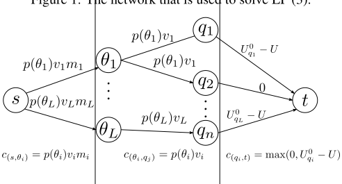
We now show that LP (3) can also be solved using a network flow approach. Specifically, given a value U for the objective, we can compute a feasible solution that attains this objective value (if it exists), as follows. We construct a network consisting of a directed graph (V,E) and capacities ce on the edges, as follows (see also Figure 1).
Definition 2 (Test network). Given an instance of the test game and a value U, construct a network as follows. Let V = {s} ∪ Θ ∪ Q ∪ {t} and E = ({s} × Θ) ∪ (⋃θ∈Θ{θ} × Hθ) ∪ (Q × {t}). For each edge (s, θ), let its capacity be c(s,θ) = p(θ)vθmθ. For each edge (θ, q) (with q ∈ Hθ), let its capacity be c(θ,q) = p(θ)vθ. Finally, for each edge (q, t), let its capacity be c(q,t) = max(0, U 0 q -U).
Proposition 4. The test network has a feasible flow that saturates all the edges in Q × {t} if and only if LP (3) has a feasible solution with value U.
Proof. If the test network has a feasible flow f that saturates all the edges in Q × {t}, then consider the solution to LP (3) where zθ,q = f(θ,q)/c(θ,q), so that clearly 0 ≤ zθ,q ≤ 1. Because the Q × {t} edges are saturated, we have that for each q ∈ Q, ∑θ:q∈Hθ p(θ)vθzθ,q = ∑θ:q∈Hθ f(θ,q) = max(0,U 0 q - U) ≥ U 0 q - U, which implies U ≥ U 0 q - ∑θ:q∈Hθ p(θ)vθzθ,q. For each θ ∈ Θ, because of the capacity constraint on edge (s, θ), we have ∑q∈Hθ zθ,q = (1/(p(θ)vθ)) ∑q∈Hθ f(θ,q) ≤ (1/(p(θ)vθ))f(s,θ) ≤ (1/(p(θ)vθ))p(θ)vθmθ = mθ. Hence, we have a feasible solution to LP (3) with objective value U.
Conversely, if we have a feasible solution to LP (3) with objective value U, then set: (1) f(θ,q) = 0 if U 0 q ≤ U; (2) otherwise, set f(θ,q) = U 0 q -U ∑θ:q∈Hθ p(θ)vθzθ,q zθ,qc(θ,q). To satisfy the flow constraints, this implies f(s,θ) = ∑q∈Hθ f(θ,q) and f(q,t) = ∑θ:q∈Hθ f(θ,q). We now check that the capacity constraints hold. By the first constraint in the LP, we have U 0 q -U ∑θ:q∈Hθ p(θ)vθzθ,q ≤ 1 so f(θ,q) ≤ zθ,qc(θ,q),
position [Birkhoff, 1946]; similar techniques are used in the context of security games [Korzhyk et al., 2010].
and because zθ,q ≤ 1 we have that the capacity constraints on the ⋃θ∈Θ{θ} × Hθ edges are satisfied. Then, we have f(s,θ) = ∑q∈Hθ f(θ,q) ≤ ∑q∈Hθ zθ,qc(θ,q) = p(θ)vθ ∑q∈Hθ zθ,q ≤ p(θ)vθmθ = c(s,θ) by the second constraint of the LP. Finally, for any q ∈ Q, there are two cases: (1) if U 0 q ≤ U, then we have f(q,t) = ∑θ:q∈Hθ f(θ,q) = 0; (2) if U 0 q > U, we have f(q,t) = ∑θ:q∈Hθ f(θ,q) = U 0 q -U ∑θ:q∈Hθ p(θ)vθzθ,q ∑θ:q∈Hθ zθ,qc(θ,q) = U 0 q - U. So the Q × {t} edges are exactly saturated.
We can do a binary search for the optimal value of U to the desired level of precision. 3 The proof of Proposition 4 shows us how to find the test taker's strategy corresponding to a particular flow.
7.3 ADirect Algorithm for Identifying the Tester's Strategy
We now give a direct algorithm (Algorithm 1) that, given an equilibrium strategy for the test taker, computes an equilibrium strategy for the tester. This also allows us to prove that there always exists such a strategy where the tester uniformly randomizes over a subset of the questions (rather than, for example, placing high probability on a question that is hard for many types and low, but nonzero, probability on a question that is hard for fewer types).
Algorithm 1 Input: A test game with t = 1 and an optimal primal solution (U, (zθ,q)) to LP (3).
- 1: T ← {q | U 0 q - ∑θ:q∈Hθ p(θ)vθzθ,q = U} 2: S ← {θ : ∑q∈Hθ∩T zθ,q <mθ} 3: while S has an unmarked element do 4: θ ← an unmarked element from S 5: for all q ∈ Hθ ∩ T and zθ,q < 1 do 6: S ← S ∪ {θ′ ∈ Θ : q ∈ Hθ′ ∧ zθ′ ,q > 0} 7: T ← T \ {q} 8: end for 9: mark θ 10: end while 11: return the uniform distribution over T
To prove the correctness of Algorithm 1, we first introduce the following two lemmas.
Lemma 1. At every point in Algorithm 1, T is nonempty.
3 If an exact solution is desired, we can use a similar construction to reduce to the minimax network flow problem [Han, 1997], where the goal is to compute a maximum flow that minimizes maxe∈E′ fe for some distinguished set of edges E′ ⊆ E. To do so, first (assuming w.l.o.g. U 0 q1 ≤ U 0 q2 ≤ U 0 qn ) we use our algorithm above to find out in which interval [U 0 qi , U 0 qi+1 ] the optimal U lies. Then, we modify the network by setting c(q,t) = max(0,U 0 q - U 0 qi+1 ) and find a flow that saturates these edges. We consider the residual graph consisting of the remaining capacities, and again adjust the capacities c(q,t) from 0 to U 0 qi+1 -U 0 qi whenever U 0 q ≥ U 0 qi ; finally, we can call a minimax network flow solver on this network with E′ = Q×{t}. However, as we are not aware of any such solvers, in our experiments we focus on the approach based on binary search.
(a) Increasing n with
L = 150 and mmax = 6.
(b) Increasing L with
n = 150 and mmax = 6.
(c) Increasing mmax with
n = L = 150.
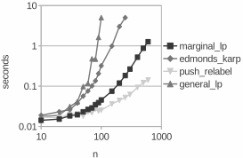
(d) Increasing n with L = n
and mmax = ⌊√n⌋.
Figure 2: Runtime for solving for an optimal tester strategy in one-question tests.
Proof. T is non-empty initially, because otherwise U would clearly be suboptimal. Let T0 denote that initial T. Suppose that at some point, all questions in T0 are deleted. We will show how to construct an alternative solution (z′θ,q ) such that for each q ∈ T0, we have ∑θ∈Θ:q∈Hθ p(θ)vθz′θ,q > ∑θ∈Θ:q∈Hθ p(θ)vθzθ,q. This would then allow us to reduce U, contradicting its optimality.
We initialize z′θ,q = zθ,q for all θ, q ∈ T0 ∩ Hθ, and z′θ,q = 0 otherwise. Then, we will adjust the z′θ,q for q ∈ T0 in the same order in which these q were eliminated from T. We maintain the property that, if q is the latest question for which we have adjusted the z′θ,q , then for all θ ∈ Sq (where Sq is the subset S in the algorithm after eliminating q), we have ∑q∈Hθ z′θ,q < mθ. This property holds initially by the initialization of S. When we reach q ∈ T0, because it was eliminated, there is a θ ∈ S such that z′θ,q < 1. Let ϵ = (1 - z′θ,q )/2. Then, let z′θ,q ← z′θ,q + ϵ and, for every θ′ ∈ Θ such that q ∈ Hθ′ and z′θ′ ,q > 0, let z′θ′ ,q ← z′θ′ ,q - min(z′θ′ ,q , ϵ 2|Θ| p(θ)vθ p(θ′ )vθ′ ), thereby maintaining the property. As a result, ∑θ′′∈Θ:q∈Hθ′′ p(θ′′ )vθ′′z′θ′′ ,q will have increased by at least ϵp(θ)vθ-∑θ′∈Θ p(θ′ )vθ′ ϵ 2|Θ| p(θ)vθ p(θ′ )vθ′ = ϵp(θ)vθ|Θ| ϵ 2|Θ| p(θ)vθ > 0. Hence, at the end, for each q ∈ T0, we have ∑θ∈Θ:q∈Hθ p(θ)vθz′θ,q > ∑θ∈Θ:q∈Hθ p(θ)vθzθ,q.
Lemma 2. Let (zθ,q) be the solution to LP (3) and let T be the final subset that Algorithm 1 returns. Then for each type θ, either ∑q∈Hθ∩T zθ,q = mθ (θ memorizes as much of T ∩Hθ as possible) or ∀q ∈ Hθ ∩ T, zθ,q = 1 (θ memorizes every question in T ∩Hθ with probability 1 and will certainly pass the test). Therefore all types of test taker are best-responding.
Proof. We will show that the algorithmmaintains the following properties after initialization of T and S. (1) Any type θ ∈ Θ for which ∑q∈Hθ∩T zθ,q <mθ is in S. (2) All marked types θ satisfy ∀q ∈ Hθ ∩ T, zθ,q = 1. From this, the lemma follows, because at the end of the algorithm, the condition for the while loop must be false, so every type must be either not in S, in which case the first condition in the lemma holds, or marked, in which case the second condition holds.
Clearly (1) and (2) hold after initialization. For any θ, the only way in which ∑q∈Hθ∩T zθ,q can decrease is if some q ∈ Hθ with zθ,q > 0 is removed from T; but in that case, in the preceding line of the algorithm, θ will have been added to S. This proves (1) is maintained. When some θ is marked, all q ∈ Hθ such that zθ,q < 1 have just been removed from T. This proves (2) is maintained.
Theorem 3. Let (zθ,q) be the solution to LP (3) and (xq) the uniform distribution over the set T returned by Algorithm 1. Then ((xq), (zθ,q)) constitute an equilibrium. 4
Proof. By Lemma 1, (xq) is a valid strategy. By the initialization of T, T can ever only include questions that give the tester the maximum utility U. Finally, Lemma 2 shows that all test taker types are best-responding.
8 Experiments
In this section, we describe experiments that we performed to see how different algorithms scale. We also show how the optimal test strategy outperforms simple test strategies, such as drawing questions uniformly at random.
8.1 Tests of Size 1: Scalability
We first restrict our attention to single-question test games, in which we can evaluate all our algorithms at once. We consider four different algorithms. We use CPLEX (out-of-thebox) to solve (1) the general LP (1) and (2) the one-question marginal-probabilities LP (3). Also, we use the network-flow approach from Definition 2 with binary search on U to a precision of 10-8 using (3) Edmonds-Karp [Edmonds and Karp, 1972] and (4) Push-Relabel [Goldberg and Tarjan, 1988], in each case combined with Algorithm 1 to compute the tester's optimal strategy.
In particular, we use CPLEX 10.010 and the boost 1.46.1 C++ library for Edmonds-Karp and Push-Relabel. Our machine has an Intel i7-2600 3.40GHz CPU and 8GB memory.
For each experimental data point, we specify three parameters: the number of questions n, the number of types L (|Θ| = L), and the maximum memory size mmax. We always set bmax, the maximum size of any Hθ, to 2mmax. Given those parameters, a test game instance is randomly generated as follows: for each θ ∈ Θ, draw mθ uniformly from 1 to mmax; draw |Hθ| uniformly from mθ to bmax; generate Hθ by drawing |Hθ| elements from Q uniformly; and draw wθ = p(θ)vθ uniformly from [0, 1] (these two factors always appear together). For each data point, we generate 5 test game instances and compute the average running time for each algorithm. We set a timeout of 5 seconds for each instance.
4 By complementary slackness, this also means they constitute optimal primal and dual solutions to our LPs.
Figures 2(a), 2(b), and 2(c) show how the algorithms scale in n, L, and mmax, respectively, holding the other parameters fixed. (Note the logarithmic scales on Figure 2(c).) None of the algorithms have trouble scaling in n alone. EdmondsKarp does not scale very well in L and mmax, and the general LP scales particularly poorly in mmax. The marginal LP and particularly push-relabel always scale very well.
In fact, these experiments indicate increasing a single parameter by itself never leads to truly hard instances. For n eventually many of the questions become irrelevant (not hard for any type). For L and mmax, eventually it becomes optimal to randomize uniformly over all questions. Thus, to identify more challenging instances, multiple parameters need to increase simultaneously, as we do in Figure 2(d) (note again the logarithmic scales). Push-relabel performs best.
8.2 Tests withMultiple Questions: Scalability
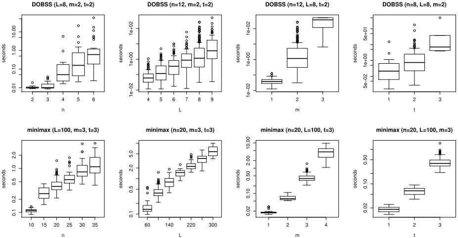
When the test can contain more than one question, the only algorithm that we have provided is our general LP (1). We compare this with the standard solver for Bayesian Stackelberg games, DOBSS [Paruchuri et al., 2008] (using the same version of CPLEX). The machine we use and the way we generate test game instances (other than the number of questions) remain the same as in the previous subsection.
Figure 3 shows that DOBSS scales quite poorly in all parameters, especially in mmax and t. As might be expected when solving MIPs, the runtime varies dramatically even for instances of the same size, as indicated by the many outliers in the plots. Our general LP (1), on the other hand, scales much better in n,L. It does still struggle when scaling mmax and t (though it outperforms DOBSS). This is expected because the size of the LP grows exponentially in those parameters.
8.3 Tester Utility
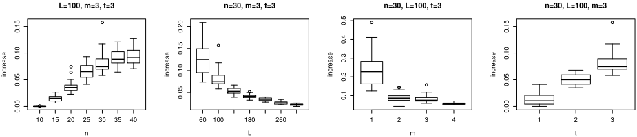
One may wonder whether computing a game-theoretically optimal strategy is worth the effort; maybe a simple heuristic performs almost as well. To assess this, we have compared our optimal test strategies to (1) the optimal strategy under the assumption that test takers do not memorize anything, and (2) choosing t questions uniformly at random from all questions. We generated all the test game instances as before. (1) performed exceedingly poorly, many factors worse than the optimal strategy. (2) performed decently and so we only present results comparing to (2).
As Figure 4 indicates, the performance increase drops when L and m increase, and it increases when n and t increase. This is a natural consequence of the way we generate the test game instances. The larger L and m are, the more equivalent subsets of questions are likely to be as the hardness sets start to cover the questions more uniformly; on the other hand, the opposite is true for n (for example, with large n, some questions may not be hard for any type and so a waste to test) and t (presumably because as t grows it becomes more important to pick questions that expose weaknesses of different types).
| bounded mmax | unbounded mmax | |
|---|---|---|
| t = 0, 1 | P | P |
| bounded t ≥ 2 | P | coNP-c |
| unbounded t | NP-c | coNP-h and NP-h |
All in all, the performance of the uniform strategy is quite decent. We suspect, though, that the way we construct the test game instances, which assumes that each question has the same probability to be hard for a test taker, favors the uniform strategy. In reality, we expect there to be some correlationthat is, a question that is hard for one type is more likely to be hard for another type as well-and presumably the uniform strategy is less effective in this context. Preliminary experiments on highly structured instances with this property confirm this intuition.
9 Conclusion
Table 1 summarizes our complexity results. Our work is only a small first step in the design of algorithms for gametheoretically optimal design of tests. Future research could focus on identifying other tractable cases. For example, in practice, one would expect the Hθ sets to exhibit structure that may be exploited algorithmically. Another direction is to generalize beyond tests whose only outcomes are pass and fail. From a practical perspective, it is also important to develop methodology to obtain the statistical information about test taker types that is needed as input to our algorithms. Perhaps even better than a two-phase approach, in which we first estimate this information and then run our algorithm, would be a true online-learning approach, where we update our testing strategy as additional test takers take our tests.
Acknowledgments
We thank ARO and NSF for support under grants W911NF12-1-0550, W911NF-11-1-0332, IIS-0953756, and CCF1101659.
A Counterexample to Zero-SumEquivalence when the Test Taker is Stackelberg Leader
Let Q = {q1, q2}, Θ = {θ1, θ2}, Hθ1 = Hθ2 = Q, mθ1 = mθ2 = 1, p(θ1) = p(θ2) = 1/2, t = 1, vθ1 = 100, vθ2 = 1, ωθ1 = 1, and ωθ2 = 100. If the tester is the leader, then it is optimal for her place probability 1/2 on each question (and so, by Proposition 1, this is also optimal in the zero-sum version of the game). This results in an expected utility of 0.5 for a test taker of type θ1, and one of 50 for a test taker of type θ2-so an expected utility of 25.25 for the test taker ex ante.
However, if the test taker can commit to a strategy in the Bayesian game ex ante (before learning his type), then he can commit to memorize conditionally on the type as follows: Mθ1 = {q1} and Mθ2 = {q2}. Because the tester cares more about failing θ1, she will test q2. This results in an ex ante expected utility of (1/2) · 100 = 50 for the test taker, which is more than the 25.25 from the strategy in the regular version.
@inproceedings{ijcai2013p47,
  title     = {Game-Theoretic Question Selection for Tests},
  author    = {Li, Yuqian and Conitzer, Vincent},
  booktitle = {Proceedings of the Twenty-Third International Joint Conference on
               Artificial Intelligence, {IJCAI-13}},
  publisher = {AAAI Press / International Joint Conferences on Artificial Intelligence},
  editor    = {Francesca Rossi},
  pages     = {254--261},
  year      = {2013},
  month     = {8},
  url       = {https://ijcai.org/proceedings/2013/47},
}
TY - CPAPER TI - Game-Theoretic Question Selection for Tests AU - Li, Yuqian AU - Conitzer, Vincent T2 - Proceedings of the Twenty-Third International Joint Conference on Artificial Intelligence, IJCAI-13 PB - AAAI Press / International Joint Conferences on Artificial Intelligence PY - 2013 SP - 254 EP - 261 UR - https://ijcai.org/proceedings/2013/47 ER -Copied
Machine-readable versions of this paper, for tools and AI agents:





