Probabilistic Inference Based Message-Passing for Resource Constrained DCOPs

1 Introduction

Distributed constraint optimization (DCOP) is a general framework for coordinated decision making by a team of agents [Yokoo et al., 1998; Mailler and Lesser, 2004; Modi et al., 2005; Petcu and Faltings, 2005]. DCOPs have been used to model several multiagent coordination problems [Maheswaran et al., 2004; Kumar et al., 2009; L´eaut´e and Faltings, 2011; Zivan et al., 2014]. In DCOPs, agents control a set of variables with constraint or utility functions defined over subsets of variables. The task for agents is to assign values to variables to maximize the global utility using only local coordination among them.

In several real world applications, agents consume multiple shared resources with limited capacity. For e.g., in distributed meeting scheduling, agents' schedule is constrained by their travel budget; in sensor networks, sensors may have limited battery. The coordination problem is now to optimize the global objective, while also respecting the resource limit for each resource. To address such settings, the framework of resource-constrained DCOPs (RC-DCOPs) has been developed [Bowring et al., 2006; Matsui et al., 2008; Bowring et al., 2009; Matsui et al., 2011], and has been uti-

Pradeep Varakantham

School of Info. Systems Singapore Management Univ. pradeepv@smu.edu.sg

lized in applications such as distributed management of smart grids [Kumar et al., 2009; Matsui and Matsuo, 2012].

RC-DCOPs have been solved by extending complete and optimal DCOP search algorithms such as ADOPT [Modi et al., 2005; Bowring et al., 2006; Matsui et al., 2008], and by adding support for resources to optimal dynamic programming based DPOP algorithm [Petcu and Faltings, 2005; Kumar et al., 2009; Matsui et al., 2011]. However, progress remains slow for developing approximate solvers for RCDCOP that can provide scalable and good quality solutions in the presence of resource constraints. We show empirically that adding resources as a generic n-ary constraint to be solved using state-of-the-art approximate solvers such as max-sum (MS) [Stranders et al., 2009] makes the algorithm unstable leading to high failure rate; implying that no resource-feasible solution was returned by the algorithm. Therefore, our work develops a message-passing algorithm that explicitly addresses resource constraints, is guaranteed to converge, has low failure rate and provides high quality solutions over a range of benchmarks when compared against an efficient centralized constraint solver [de Givry et al., 2005; Allouche et al., 2010].

Our work is motivated by the recently developed connections between decision making and probabilistic inference. Such planning-as-inference paradigm allows adoption of well known inference techniques such as expectation-maximization (EM) [Dempster et al., 1977] for single agent planning [Toussaint and Storkey, 2006; Toussaint et al., 2008] and also multiagent planning [Kumar et al., 2011b]. Such inference based approach has also been applied to the problem of MAP estimation in graphical models [Kumar and Zilberstein, 2010], which is (almost) equivalent to the DCOP problem [Kumar et al., 2011a]. We extend the approach of [Kumar and Zilberstein, 2010] to RC-DCOPs. However, addressing resource constraints within the EM framework proves challenging as unlike the setting in [Kumar and Zilberstein, 2010], EM for RC-DCOP does not admit closed form solutions. Therefore, we combine several tools from convex optimization machinery (such as dual optimization, block coordinate descent) and algebra (polynomial root finding) in a novel way to derive the EM algorithm for RC-DCOPs. EM is easily implementable using local message-passing among agents, and is highly scalable. Unlike approaches such as MS, EM is guaranteed to converge. Empirically, we show that EM provides similar or better quality than MS, has low failure rate even under tight resource constraints and also proves highly competitive to an efficient centralized constraint solver.

2 The DCOP Framework

This section introduces the DCOP and the resource constrained DCOP (RC-DCOP) [Bowring et al., 2006; Matsui et al., 2008] frameworks. A DCOP is defined using the tuple 〈X , D, Θ〉. The set X ={x1, . . . , xn} is a set of n variables; D={D1, . . . ,Dn} is the (finite) domain of possible values a variable can take. The set Θ={. . . , θij, . . .} is the set of utility or constraint functions. A constraint function between variables xi and xj is defined as θij : Di ×Dj → ℜ. We assumed w.l.o.g. that each function involves two variables.

The DCOP framework can be represented using a constraint network G=(V, E) as follows. There is a node i for each variables xi. For each constraint θij , we create an edge between the nodes i and j in the graph. The objective is to find the joint variable assignment to solve:

A key property of DCOPs is that there is an agent associated with each node of the constraint graph. An agent is only aware of its shared constraints with neighbor agents. Thus, there is no centralized view of the whole problem, requiring local message-passing based coordination.

Resource Constrained DCOPs (RC-DCOPs) add support for resources to DCOPs. They include a set R of resources and a set U of requirements. The set R={r1, . . . , rm} is the set of m resources. Each resource ri has a fixed capacity C(ri). The set U is a collection of resource utilization functions ui(·) for each agent i defined as ui :R×Di→ℜ+. The RC-DCOP framework solves the same problem as (1) with the added resource constraints as below:

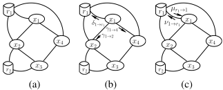
We define a resource-augmented constraint network (RACN) for a RC-DCOP by creating one node for each of the m resources. For e.g., in figure 1(a), we have four agents x1 to x4, and two resources r1 and r2. We say that an agent i is involved in resource constraint r if ∃xi ∈Di : ui(r, xi) > 0. Using this notion, we create an edge between a resource r and all the agents that are involved in r. In figure 1(a), resource r1 involves three agents x1, x2 and x4 denoted using dotted

Table 1: Quadratic programming based relaxation of RCDCOP

edges. Notationally, i and j denote agents and their corresponding variables xi and xj in RACN (see fig. 1); symbol r is used to index resources. Let Nb(i) denote the agents that are immediate neighbors of agent i. For e.g., Nb(1)={2, 4} in fig. 1. Let Nr(i) denote resources that are connected to the agent i (e.g., Nr(2)={r1, r2} in fig. 1). For a resource r, Nb(r) denotes agents that are connected to it (e.g., Nb(r2)={2, 3}).

3 Continuous Relaxation of RC-DCOP

In this section, we first present a continuous relaxation of the DCOP and RC-DCOP problems. The continuous relaxation is essentially a quadratic program (QP) for solving the DCOP problem [Ravikumar and Lafferty, 2006]. The basis for this QP lies in the near-equivalence of the DCOP problem and MAP estimation in graphical models [Ravikumar and Lafferty, 2006; Kumar et al., 2011a]. We associate a probability distribution pi(xi) with each variable xi in the DCOP. We can then write the following QP:

The following result proved in [Ravikumar and Lafferty, 2006] shows that such a QP relaxation is tight.

Theorem 1. Let f ⋆ dcop denote the optimal objective for the DCOP problem (1) and f ⋆ qp denote the optimal objective for the QP in (3). Then we have f ⋆ dcop =f ⋆ qp .

Therefore, optimally solving the QP (3) in a distributed manner will also solve the DCOP problem. However, this QP is non-convex, therefore, convergence to the global optimum is not guaranteed.

RC-DCOP Relaxation Based on the QP formulation of the DCOP problem, we now present a QP formulation of the RCDCOP problem in table 1. The key addition in the QP for RCDCOP are constraints (6) for each resource r. This constraint says that for each resource r, the expected consumption of this resource by all the agents (=Nb(r)) must be less than the resource's capacity C(r). Notice also that all these constraints are linear in QP parameters pi, which would be advantageous later.

Theorem 2. Let f ⋆ rcdcop denote the optimal objective for the RC-DCOP problem (1) subject to constraints (2) and f ⋆ qprc denote the optimal objective for the QP in table 1. Then we have f ⋆ qprc ≥ f ⋆ rcdcop .

We omit the formal proof for space reasons. It is easy to show the connection of the QP in table 1 with the LP relaxation of the knapsack problem.

Our goal in this work is to solve the QP relaxation of RCDCOP in table 1 in a distributed manner. We achieve this goal via the following:

• We first transform the RC-DCOP problem to that of likelihood maximization (LM) in a mixture of Bayesian networks. The likelihood maximization problem is exactly equivalent to solving the QP in table 1.
• We then use the well known Expectation-Maximization (EM) framework [Dempster et al., 1977] to maximize the likelihood in the Bayes net mixture. However, the M-step in this EM formulation does not admit a closed form solution. Therefore, we use tools from convex optimization such as block coordinate descent, and tools from algebra such as polynomial root finding to develop a messagepassing algorithm to efficiently perform the M-step.

Once the EM algorithm has converged, we use a similar message-passing based rounding technique proposed in [Ravikumar and Lafferty, 2006] to extract an integral variable assignment from the QP solution.

4 Expectation-Maximization For RC-DCOPs

In this section, we follow the similar strategy as in [Kumar and Zilberstein, 2010] to recast the RC-DCOP as a likelihood maximization problem. The key idea is to decompose the constraint network into a mixture model of simpler Bayes nets with many hidden variables - all the variables xi of the RC-DCOP. To incorporate the constraint functions θ's of RCDCOP and achieve equivalence between the likelihood and the RC-DCOP objective, a special binary reward variable ˆ θ is introduced with its conditional distribution proportional to potentials θ.

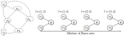
For each edge (i, j) in the constraint network, we create a depth-1 Bayes net (BN). Notice that we do not consider edges between resources and agents during this process. Each Bayes net consists of a binary reward variable ˆ θ with its parents being the variables xi and xj. Fig. 2(a) shows the RACN for a RC-DCOP instance over four variables. Fig. 2(b) shows the equivalent mixture of Bayes nets for each of the four agent-toagent edges in this network. The mixture random variable l (with domain being agent-agent edge set E), is used to identify the Bayes nets for the corresponding edge. It has a uniform distribution (= 1/|E|).

The parameters to estimate in this mixture are the probabilities pi(xi) for each node xi. Intuitively, these are the same as the variables in the QP of table 1. Furthermore, different Bayes nets share the same parameter pi for any common variable xi. E.g., variable x2 in figure 2(b) is involved in two Bayes nets for l=(1, 2) and l=(2, 3). Therefore, p2(x2) is the same for these two Bayes nets. The space Θ of all the valid parameters is specified by the following linear constraints:

Non-negativity of each pi is also included in Θ. Therefore, the constraint on valid parameters in this BN mixture replicate those of in table 1. Next we set the conditional probability distribution of the variable ˆ θ for each of the Bayes nets. For a BN l involving variables xi and xj, it is set as follows:

where θmax and θmin are the maximum and minimum value over all constraint functions. The probabilities ˆ θxi,xj are essentially normalized constraint functions θij for the RC-DCOP instance.

Theorem 3. For each BN l, let the CPT of binary reward variable ˆ θ be set as per (7). Then maximizing the likelihood Lp = P(ˆ θ = 1; p) of observing the reward variable in the mixture of Bayes nets is equivalent to solving the QP relaxation of RC-DCOP in table 1.

The proof is similar to the one in [Kumar and Zilberstein, 2010] that shows the equivalence of likelihood maximization and the QP formulation (3) for DCOP. The only difference in our case is that the space of possible parameters Θ includes resource constraints, which makes the likelihood maximization approach applicable to RC-DCOPs.

4.1 Expected Log-Likelihood

To derive the EM algorithm for BN mixture of figure 2(b), we assume that only the reward variable ˆ θ = 1; rest of the variables are hidden. The full-joint for a BN l is given as:

The EM algorithm maximizes the following expected loglikelihood, Q(p, p⋆ ), w.r.t.p⋆ iteratively [Kumar and Zilberstein, 2010; Dempster et al., 1977]:

where xl1 and xl2 denote the two variables that are involved in the BN l, p denotes the previous iteration's parameters and p⋆ denote the new parameters to be optimized. We take the log of (8), and simplify Q(p, p⋆ ) as follows:

In the above expression, we have ignored terms independent of p⋆ . We simplify the above expression by grouping together terms for each variable xi:

Using the above expression, the M-step involves solving the following convex optimization problem (minus sign used to make it a minimization problem):

4.2 Maximizing Expected Log-Likelihood

In this section, we detail how to solve the convex optimization problem (11). Because of the complicating resource constraints (13), this problem does not admit a closed form solution unlike the case in [Kumar and Zilberstein, 2010]. Therefore, we use several tools from convex optimization and algebra to develop a message-passing algorithm for this problem. Our high level approach is as follows:

• We write the dual of problem (11). The dual has simpler structure than the original problem, making optimization easier. Furthermore, as (11) is a convex optimization problem, there is no duality gap implying optimal dual quality equals optimal of (11) [Bertsekas, 1999].
• To optimize the dual, we use results from convex optimization [Bertsekas, 1999] that guarantee that a block coordinate descent (BCD) strategy wherein we fix all the dual variables except one, and then optimize the dual over the one variable is guaranteed to converge to the optimal dual solution. The BCD strategy gets translated into message-passing over the RACN.

Dual of (11): We first write the Lagrangian function for problem (11) by introducing dual variables λ,µ for constraints (12), (13) respectively:

The dual function is q(λ,µ)=minp⋆ L(p⋆ , λ,µ). It is found by setting derivatives of L(p⋆ , λ,µ) w.r.t. each p⋆i to zero. Upon simplification, the dual is given as:

Optimizing the dual (15): We now detail the problem of maximizing the dual: maxλ,µ q(λ, µ). Notice also the fact that the domain of function q(·) includes only those λ, µ where q(·) is defined and is greater than -∞ [Bertsekas, 1999]. We also have each variable µ ≥ 0 [Bertsekas, 1999]. These facts will be exploited later.

Block Coordinate Descent (BCD) Consider the following iterative strategy to maximize (15). We choose an arbitrary dual variable, say λi, fix all other variables, and optimize the function q(·) w.r.t.the chosen variable (λi). In general, this strategy is not guaranteed to converge to the optimal solution. However, the function q(λ, µ) satisfies additional properties which guarantee that the BCD approach will converge to the optimal. These conditions are a) q(·) is continuously differentiable over its domain; b) q(·) is strictly concave w.r.t.each dual variable λi and µr due to the presence of log terms in (15), resulting in a unique solution for each BCD iteration [Bertsekas, 1999, Proposition 2.7.1].

We now detail optimization over a single λi variable, fixing all other variables. This can be done by setting partial derivative w.r.t. λi of q(·) to zero, resulting in:

Roots of rational functions: Notice that (16) is a rational function in λi, and solving for λi will result in multiple values of λi. This complicates the BCD approach which requires a unique value for λi. Fortunately, we show that despite multiple λis satisfying (16), there is one and only one λi that is applicable in our approach. Essentially, we show that there is just one λi for which the dual function q(·) in (15) is defined, for every other possible λi, q(·) becomes undefined as it involves taking the log of a negative quantity. We start by considering a rational function of the form as:

where index T denotes total number of terms, at > 0, bt ≥ 0 ∀t, and c > 0. Eq. (16) fits such a rational function categorization as numerator is positive and all variables µ are also positive. We now analyze the roots of g(x)=0. Let us consider an ascending order over the terms bt such that b1 is smallest and bT is the largest. For simplicity, assume that each of bt is different and positive (> 0).

Theorem 4. The rational function g(x) of the form (17) has exactly one root in each interval (-bt+1,-bt) ∀t=1 to T-1 and exactly one root in the interval (-b1,∞).

Proof sketch. Notice that discontinuity in the function g(x) occurs only at points -bt ∀t. Consider the interval [-bt+1+ ϵ,-bt-ϵ] for any ϵ>0 such that -bt+1+ϵ<-bt. We have:

As ϵ → 0, then we have g(-bt+1 + ϵ) → +∞ and g(-bt-ϵ) → -∞. We also know that g(x) is continuous and monotonically decreasing (using the first derivative test) in the interval [-bt+1+ϵ,-bt-ϵ]. Therefore, we can deduce that g(x) crosses the horizontal axis y=0 exactly once in this interval. This proves the first part of the theorem.

Algorithm 1: solveRCDCOP(θ, u)

Using similar argument as above, we can show that there is no root in the interval (-∞,-bT ) (proof omitted). Given that the total number of roots of g(x) is T and total number of intervals (-bt+1,-bt) are T - 1, it implies that there is exactly one root in the remaining interval (-b1,∞).

We now relate the above theorem to our problem of determining a unique solution of (16). From analyzing log terms in (15), we have:

The term maxxi -∑r µrui(r, xi) is equivalent to the term -b1 used in the theorem 4. Therefore, we require that a feasible λi must lie in the interval (-b1,∞). Using theorem 4 we already know that there is just one root for any rational function g(x) in this range. And this unique root in the interval (-b1,∞) is the valid solution of (16) used by BCD approach.

Maximizing (15) w.r.t.µr requires finding the unique value of µr from the following equation:

As noted before, dual variables µ must be positive. Let r denotes the largest root for the above rational function, we can show that max(0, r) is the unique solution for the BCD approach.

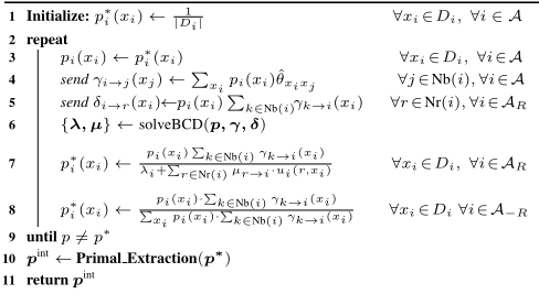
Message-passing implementation: All the steps of the EM and the BCD approach can be implemented via messagepassing over the RACN for a RC-DCOP as shown in Alg. 1 and 2. Let A=AR ∪ A-R denote the set of all agents, AR denotes agents that are directly connected to at least one resource and A-R denotes agents that do not participate in any resource constraint. The EM algorithm for RC-DCOPs is a double loop message-passing algorithm as shown in alg. 1.

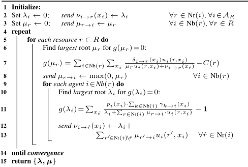
In the outer loop (lines 2-9 of algo. 1), two types of messages are passed among agents and resources, as shown in fig. 1(b) and lines 4 and 5 in algo. 1. Message γi→j (size=|Dj |) is passed from agent i to its neighbor agent j, δi→r (size=|Di|) is passed from agent i to connected resource r. In the inner loop (lines 4 to 14 in algo. 2), the steps of the BCD approach are implemented. In the inner loop, message νi→r (size =|Di|) is passed from agent i to connected resource r, µr→i (size=1)

Algorithm 2: solveBCD(p, γ, δ)

is passed from resource r to agent i. Both these message types are shown in fig. 1(c).

The core of the BCD approach is implemented in lines 5 to 12 in algo. 2. Line 6 updates the µr variable by finding the largest root of the given rational function; similarly line 10 updates the λi variable. Notice that while root finding, agents and resources use the latest µ or ν message they have received. Main idea is that whenever a variable is updated, its updated value must be communicated to all other relevant entities that depend upon the updated variable. For example, after the variable λi is updated in line 11, an updated message ν is sent to all the resources r connected to i in line 12. Convergence is detected in the inner loop if messages change by a value smaller than a given threshold.

Primal Extraction: Upon convergence, we extract the integral solution from p⋆ using a similar rounding technique as proposed in [Ravikumar and Lafferty, 2006, Theorem 3.2] by adding to it support for handling resources. This rounding technique also has a message-passing structure.

Complexity: Let m denote the maximum number of agents involved in any single resource; m′ denote the maximum number of resources any single agent is connected to. If inner loop (lines 4 to 14 in algo. 2) is run for I iterations, then total µ messages are O(mI|R|). Total number of ν messages is O(mm′ I|R|). In each outer loop iteration (lines 2 to 9 in algo. 1), the total number of messages exchanged (both γ and δ) equals to the number of edges in the RACN. The maximum size of any message (in inner or outer loop) is bounded by the maximum domain |D|max of any variable. Thus, our messagepassing approach is highly efficient and scales gracefully with the number of edges or resources in the RACN.

5 Experiments

We compare our EM approach with the popular approximate DCOP algorithm max-sum (MS). Resource constraints were encoded as n-ary constraints for MS. As both the EM and MS lack quality guarantees, we also show results against an optimal efficient constraint solver 'toulbar2' [Allouche et al., 2010]. We imposed a time limit of 1 hour for toulbar2. We used the MS implementation provided by the Frodo 2.0 software [L´eaut´e et al., 2009]. Our approach was implemented in Python and used Bisection method for root finding. We test on two benchmarks, random graphs and graph coloring.

Random graphs: We tested with 30 and 40 node graphs with domain size |Di|=5. We vary the edge density from 0.5 to 0.9 resulting in challenging problems. Each utility, θij(·, ·), is a random value between 1 and 10. Each resource constraint involved three agents. Total number of resources created were such that about 50% of all the agents were involved in at least one resource constraint. A 30 node problem had 5 resource constraints on an average, and a 40 node problem had about 7 resource constraints. The resource consumption of agents for each resource was also generated randomly between 1 to 5. We controlled the resource capacity C(r) of each resource carefully. Let Mr, mr denote the maximum and minimum amount of resource r respectively that can be consumed by all the involved agents. To control the tightness of capacity constraints, we use a parameter tr varied from 0.2 to 0.6. The capacity C(r) is set as mr+tr(Mr-mr). For each setting 〈#Nodes, edge density, resource capacity〉, we generated 4 instances.

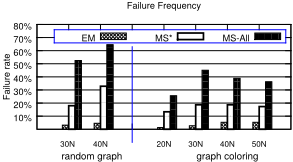
Failure rate: We first report on the failure rate of MS and EM for random graphs and graph coloring for varying node sizes in Figure 3. If a particular run of the algorithm fails to find a resource feasible solution for a given feasible instance, it is classified as a failed run. For MS, we ran it 3 times for each instance. We set 1000 iterations for each run and used the best solution over all the iterations. MS gave variable results for each run. In contrast, we ran EM just once for each instance, and EM's final solution is deterministic for a given initialization of parameters. We report two statistics for MS, the best failure rate (MS∗ in figure 3) denotes percentage of instances for whom none of MS's three runs produced a feasible solution. The 'MS-All' in figure 3 denotes the total percentage of runs where MS failed to find a feasible solution.

Figure 3 clearly shows the instability of the MS algorithm in the presence of resource constraints. Even the best failure rate of MS ('MS∗ ') was as high as 32% for 40 node random graphs. The overall failure rate of MS ('MS-All') was much higher, more than 50% for random graphs and about 40% for graph coloring problems. This shows that a significant fraction of MS's runs resulted in failure. In contrast, EM's failure rate is extremely low (less than 5%) across all the problems despite EM being run just once for each instance. These results further show that by accounting for resources explicitly, the EM algorithm is significantly more stable and better than MS across different settings.

Quality: Figure 4(a) shows (average) quality comparisons between EM and toulbar2 on common 40 node instances where both EM and toulbar2 return a resource feasible solution. The x-axis shows resource tightness varied from tr =0.2 to tr = 0.6, and edge density varied from 0.5 to 0.9. We show normalized quality for EM by assigning 1 to the quality achieved by toulbar2. As we can clearly see, EM was always able to achieve a solution very close to toulbar2. Indeed, for harder instance with higher edge density, such as 'density=0.9', EM provided better quality than toulbar2, which did not find the optimal solution within 1 hour limit. The average time required by EM was 180 sec., showing that EM was significantly faster than the toulbar2 solver.

Figure 4(b) shows (average) quality comparisons between EM, MS and toulbar2 on common instances where each algorithm found a resource feasible solution. These results also show clearly that EM always provided similar or better quality than MS. Figure 4(c) and (d) show the same previous two sets of comparisons for 30 node problems. For these problems, toulbar2 was able to achieve the optimal solution for most instances. EM achieved very close to the optimal solution. From figure 4(d) we further observe that EM provided better quality than MS.

Graph coloring: We also tested EM on graph coloring instances generated in the same fashion as [Farinelli et al., 2008]. Resource constraints are generated similarly as for random graphs. Figure 4(e) shows the results for 20 to 50 nodes and varying resource tightness tr from 0.2 to 0.6 on the x-axis. These results further show that EM is highly competitive even with a centralized solver, while having a low failure rate (less than 5%) when compared against the existing MS algorithm.

Timing results: Figure 4(f) shows the (average) runtime (in log scale) for toulbar2, EM and MS for the most challenging 40 node random graphs. The toulbar2 had a time limit of 1 hour. While MS is the fastest of all, as shown before, its solution quality is worst and failure rate high. In contrast, EM almost always converged within 3 min for all the settings and also provided comparable quality solutions to toulbar2 for higher density graphs. Therefore, EM proved very effective for these challenging problems.

6 Conclusion

We presented a promising new class of algorithms based on probabilistic inference for RC-DCOPs. We showed a close connection between likelihood maximization and RC-DCOPs, and using this connection developed the EM algorithm for RC-DCOPs. By using tools from convex optimization, we showed that EM algorithm takes a message-passing structure over the constraint network. Unlike previous approaches, such as MS, EM is guaranteed to converge. Empirically, EM had significantly lower failure rate than MS even in the presence of tight resource constraints, and proved highly competitive to a centralized constraint solver.