
Scalable Multiagent Planning Using Probabilistic Inference
Proceedings of the Twenty-Second International Joint Conference on Artificial Intelligence. Pages 2140-2145.
https://doi.org/10.5591/978-1-57735-516-8/IJCAI11-357
© 2011 International Joint Conferences on Artificial Intelligence
Abstract
Multiagent planning has seen much progress with the development of formal models such as Dec-POMDPs. However, the complexity of these models—NEXP-Complete even for two agents—has limited scalability. We identify certain mild conditions that are sufficient to make multiagent planning amenable to a scalable approximation w.r.t. the number of agents. This is achieved by constructing a graphical model in which likelihood maximization is equivalent to plan optimization. Using the Expectation-Maximization framework for likelihood maximization, we show that the necessary inference can be decomposed into processes that often involve a small subset of agents, thereby facilitating scalability. We derive a global update rule that combines these local inferences to monotonically increase the overall solution quality. Experiments on a large multiagent planning benchmark confirm the benefits of the new approach in terms of runtime and scalability.
- [Amato et al., 2010] Christopher Amato, Daniel S. Bernstein, and Shlomo Zilberstein. Optimizing fixed-size stochastic controllers for POMDPs and decentralized POMDPs. JAAMAS, 21(3):293- 320, 2010.
- [Becker et al., 2004] Raphen Becker, Shlomo Zilberstein, Victor Lesser, and Claudia V Goldman. Solving transition indepen- dent decentralized Markov decision processes. JAIR, 22:423- 455, 2004.
- [Bernstein et al., 2002] Daniel S. Bernstein, Roie Givan, Neil Im- merman, and Shlomo Zilberstein. The complexity of decentral- ized control of Markov decision processes. MOR, 27:819-840, 2002.
- [Bertsekas, 1999] Dimitri P. Bertsekas. Nonlinear Programming. Athena Scientific, Cambridge, MA, USA, 1999.
- [Boutilier, 1999] Craig Boutilier. Sequential optimality and coordi- nation in multiagent systems. In IJCAI, pages 478-485, 1999. IJCAI
- [Dempster et al., 1977] Arthur P. Dempster, Nan M. Laird, and Donald B. Rubin. Maximum likelihood from incomplete data via the EM algorithm. Journal of the Royal Statistical society, Series B, 39(1):1-38, 1977.
- [Ghahramani and Jordan, 1995] Zoubin Ghahramani and Michael I. Jordan. Factorial hidden Markov models. In NIPS, volume 8, pages 472-478. MIT Press, 1995.
- [Gill et al., 2002] Philip E. Gill, Walter Murray, and Michael A. Saunders. SNOPT: An SQP algorithm for large-scale constrained optimization. SIAM Journal on Optimization, 12(4):979-1006, 2002.
- [Gmytrasiewicz and Doshi, 2005] Piotr J. Gmytrasiewicz and Prashant Doshi. A framework for sequential planning in multi-agent settings. JAIR, 24:24-49, 2005.
- [Koller and Parr, 1999] Daphne Koller and Ronald Parr. Comput- ing factored value functions for policies in structured MDPs. In IJCAI, pages 1332-1339, 1999. IJCAI
- [Kumar and Zilberstein, 2009] Akshat Kumar and Shlomo Zilber- stein. Event-detecting multi-agent MDPs: complexity and constant-factor approximation. In IJCAI, pages 201-207, 2009.
- [Kumar and Zilberstein, 2010] Akshat Kumar and Shlomo Zilber- stein. Anytime planning for decentralized POMDPs using ex- pectation maximization. In UAI, pages 294-301, 2010.
- [Lesser et al., 2003] Victor Lesser, Milind Tambe, and Charles Or- tiz Jr., editors. Distributed Sensor Networks: A Multiagent Per- spective. Kluwer Academic Publishers, Norwell, MA, USA, 2003.
- [Marecki et al., 2008] Janusz Marecki, Tapan Gupta, Pradeep Varakantham, Milind Tambe, and Mokoto Yokoo. Not all agents are equal: Scaling up distributed POMDPs for agent networks. In AAMAS, pages 485-492, 2008.
- [Nair et al., 2003] Ranjit Nair, Milind Tambe, Makoto Yokoo, David Pynadath, Stacy Marsella, Ranjit Nair, and Milind Tambe. Taming decentralized POMDPs: Towards efficient policy com- putation for multiagent settings. In IJCAI, pages 705-711, 2003. IJCAI
- [Nair et al., 2005] Ranjit Nair, Pradeep Varakantham, Milind Tambe, and Mokoto Yokoo. Networked distributed POMDPs: A synthesis of distributed constraint optimization and POMDPs. In AAAI, pages 133-139, 2005.
- [Oliehoek et al., 2008] Frans A. Oliehoek, Matthijs T. J. Spaan, and Nikos A. Vlassis. Optimal and approximate Q-value functions for decentralized POMDPs. JAIR, 32:289-353, 2008.
- [Poupart and Boutilier, 2003] Pascal Poupart and Craig Boutilier. Bounded finite state controllers. In NIPS, 2003.
- [Toussaint and Storkey, 2006] Marc Toussaint and Amos J. Storkey. Probabilistic inference for solving discrete and continu- ous state Markov decision processes. In ICML, pages 945-952, 2006.
- [Toussaint et al., 2008] Marc Toussaint, Laurent Charlin, and Pas- cal Poupart. Hierarchical POMDP controller optimization by likelihood maximization. In UAI, pages 562-570, 2008.
- [Varakantham et al., 2009] Pradeep Varakantham, Jun young Kwak, Matthew E. Taylor, Janusz Marecki, Paul Scerri, and Milind Tambe. Exploiting coordination locales in distributed POMDPs via social model shaping. In ICAPS, 2009.
- [Witwicki and Durfee, 2010] Stefan J. Witwicki and Edmund H. Durfee. Influence-based policy abstraction for weakly-coupled Dec-POMDPs. In ICAPS, pages 185-192, 2010.
References were extracted automatically from the PDF and may contain errors.
Full text extracted automatically from the PDF; figures, tables and equations may differ. The PDF is the version of record.
1 Introduction
Sequential multiagent planning under uncertainty enables multiple cooperative agents, each with its own actions and observations, to operate autonomously in a shared environment and achieve common objectives. A number of formal frameworks have been developed to tackle such planning tasks, including multiagent MDPs [Boutilier, 1999], decentralized MDPs and POMDPs (Dec-POMDPs) [Bernstein et al., 2002]. Many problems such as multi-robot coordination [Becker et al., 2004; Oliehoek et al., 2008], broadcast channel protocols [Bernstein et al., 2002] and target tracking by a team of sensors [Nair et al., 2005] can be modeled as a Dec-POMDP. However, high complexity-NEXP-Complete even for two agents-has limited scalability [Bernstein et al., 2002].
Many recent attempts to increase the scalability of planners w.r.t. the number of agents impose restrictions on the allowed interactions among the agents such as transition independence [Becker et al., 2004; Nair et al., 2005], weak-coupling among agents that is limited to certain states [Varakantham et al., 2009], and directional transition dependence [Witwicki and Durfee, 2010]. Instead of defining yet another restricted
Marc Toussaint
Dept. of Mathematics and Computer Science, FU Berlin marc.toussaint@fu-berlin.de
model, we ask the following question: Is there a general characterization of the interaction among agents that when present in any multiagent planning model leads to a relatively scalable approximate algorithm? In this work, we characterize a class of such agent interactions and derive a scalable algorithm to solve models that belong to this class. Thus, our algorithm offers a general recipe in that certain steps are implemented in a way specific to the model at hand. In fact, these steps are easy to implement for the problems we target.
Our approach is based on reformulating the planning problem as likelihood maximization in a mixture of dynamic Bayes nets. This is inspired by recent advances in planning by probabilistic inference [Toussaint and Storkey, 2006; Toussaint et al., 2008]. Kumar and Zilberstein [2010] applied this planning-by-inference approach to two-agent planning problems. While our approach is also based on the Expectation-Maximization (EM) framework [Dempster et al., 1977] to maximize likelihood, the significant contribution is a novel characterization of general constraints that enables our method to scale far beyond two agents. Another key result is that in every model that satisfy these constraints, the E-step decomposes into a set of feasible inference queries in small components of the model. This facilitates the development of a scalable, distributed message-passing implementation of EM, ideal for large multiagent planning problems.
We show that the following common multiagent planning models fulfill our constraints: transition-independent DecMDPs [Becker et al., 2004], Network-Distributed POMDPs (ND-POMDPs) [Nair et al., 2005] and Transition-Decoupled POMDPs [Witwicki and Durfee, 2010]. We experiment on a realistic target tracking problem in sensor networks [Lesser et al., 2003] and show that EM easily scales up w.r.t. the number of agents. It also produces better results than a state-of-the-art industrial nonlinear programming solver [Gill et al., 2002].
2 Multiagent planning model
A multiagent planning problem with N cooperative agents can be modeled as a Dec-POMDP [Bernstein et al., 2002]. We denote the action of the ith agent at time t by ait . The environment is modeled by stationary state transition probabilities P(st+1 | st, a1:N t ) with an initial state distribution P (s0), where st denotes the (possibly factored) joint state and a1:N t = (a1t , .., aNt ) is the joint action of all agents. At each time step, agents receive a joint reward R(st, a1:N t ). The observation of agent i is denoted by yi t , and P(y1:N t |st, a1:N t-1 ) is the joint observation probability. In this model, each agent receives only its local observation during execution time, which is a key source of complexity [Bernstein et al., 2002].
We represent each agent's policy as a bounded, finite state controller (FSC). This approach has been used successfully for both POMDPs [Poupart and Boutilier, 2003] and DecPOMDPs [Amato et al., 2010]. In this case, each agent has a finite internal memory state, qi t , which summarizes the crucial information obtained from past observations to support efficient action selection. For POMDPs, FSCs are beneficial due to their compactness compared to the full belief state. In Dec-POMDPs, it is the only approach to tackle effectively both finite and infinite horizon problems. There are other approaches based on nested agent beliefs such as the I-POMDP framework [Gmytrasiewicz and Doshi, 2005], however we do not address them in this work.
Each agent chooses actions depending on its internal state, q: P(a|q; π) = π(a, q). The internal state is updated with each new observation, by the node transition function: P (q′ |q, y; λ) = λ(q′ , q, y). Finally, ν is the initial node distribution P(q0; ν) for each agent. In sum, the FSC of the ith agent is parameterized by θi =(πi , λi , ν i ). The goal is to find parameters θ1:N for all the agents such that the value (expected discounted future return) of the joint-policy, V (θ1:N ), is maximized.
Toussaint and Storkey [2006] introduced the idea of planning in Markov decision problems by probabilistic inference. This approach recasts the planning problem as likelihood maximization in a mixture of dynamic Bayes nets (DBNs). In this mixture, there is one DBN modeling the reward emitted at each time T. An auxiliary binary reward random variable ˆ r is introduced in each DBN such that its conditional probability is proportional to the reward of the original problem, P(ˆ r = 1 | sT , aT ) ∝ R(sT , aT ). The time T itself becomes a random variable. By choosing the geometric prior P(T) = (1 - γ) γ T , the likelihood of observing ˆ r = 1 in this mixture is proportional to the value function: P (ˆ r=1; θ) = ∑T P(T)〈P(ˆ r=1 | sT , aT )〉sT ,aT | θ ∝ V (θ), where 〈· · ·〉sT ,aT | θ is the expectation w.r.t. the length-T DBN conditioned on the policy parameters θ. Therefore, the planning problem reduces to maximizing the likelihood of observing ˆ r = 1 in this mixture. A corresponding Expectation Maximization approach has been also applied successfully to POMDPs [Toussaint et al., 2008] and 2-agent Dec-POMDPs [Kumar and Zilberstein, 2010]. Our approach extends this framework, allowing us to derive an efficient algorithm for larger multiagent planning problems.
3 New approach to multiagent planning
Let us assume that the state random variable st is factored s.t. st=(s1t , ..., sMt ), which is true in several multiagent planning models such as ND-POMDPs [Nair et al., 2005] and TD-POMDPs [Witwicki and Durfee, 2010]. Without making further (conditional independence) assumptions on the problem structure, a general Dec-POMDP requires exact inference in the full corresponding (finite-time) DBNs, which would be exponential in the number of state variables and agents. Our approach relies on a general, simplifying property of agent interaction, which we later show to be consistent with many of the existing multiagent planning models.
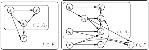
Definition 1. A value factor f defines a subset Af⊆{1, .., N} of agents and a subset Sf ⊆{1, ..,M} of state variables.
Definition 2. A multiagent planning problem satisfies value factorization if the joint-policy value function can be decomposed into a sum over value factors:
where F is a set of value factors, θf ≡ θAf is the collection of parameters of the agents of factor f, and sf ≡ sSf is the collection of state variables of this factor.
Even when the value factorization property holds, planning in such models is still highly coupled because factors may overlap. That is, an agent can appear in multiple factors as can state variables. Therefore, a value factor cannot be optimized independently. But, as we show later, it leads to an efficient Expectation Maximization algorithm. Such additive value functions have also been used to solve large factored MDPs [Koller and Parr, 1999]. We require that each value factor Vf can be evaluated using the DBN mixture based approach of Sec. 2. However, this is not a restriction, as the DBN-based approach can model arbitrary Markovian planning problems.
Theorem 1. The worst case complexity of optimally solving a multiagent planning problem satisfying the value factorization property is NEXP-Hard.
The proof of the above theorem is straightforward-any two agent Dec-POMDP is NEXP-Complete and also satisfies the value factorization property as there is only a single factor involving two agents. In fact, the work of Kumar and Zilberstein [2010] precisely addresses this case using the EM framework. Next we investigate when this property holds and when it is computationally advantageous, and establish the following result.
Theorem 2. The value factorization property holds in transition independent Dec-MDPs [Becker et al., 2004], NetworkDistributed POMDPs [Nair et al., 2005] and TransitionDecoupled POMDPs [Witwicki and Durfee, 2010]. Each value factor in these models also allows for efficient probabilistic inference in the EM framework.
The joint value is shown to be factorized based on the immediate-reward factorization in Dec-MDPs [Becker et al.,
2004] and ND-POMDPs [Nair et al., 2005]. Fig. 1 shows the plate notation for our value factor representation for both of these models. The outer plate shows a factor f and the inner plate depicts the interaction among agent parameters. We provide the EM algorithm for these two models in Sec. 3.2 and show that the inferences required by the E-step decompose along the immediate-reward factorization, which involves fewer number of agents and is thus scalable.
Our approach can also model Transition-Decoupled POMDPs (TD-POMDPs) [Witwicki and Durfee, 2010]. In this case, agents have local parameters (factored local state and rewards). However, certain features of the local state can depend on other agents' actions. This dependency among agents is described using an influence directed acyclic graph (DAG) where each node is an agent. A parent-child relationship in this DAG implies that the child's local states are controllable by the parent, but not vice-versa. An important characteristic is that given its parents' policies, an agent can compute its value function. In our representation, this translates into a value factor for each agent i, which consists of i and all its ancestors in the DAG. The joint-value decomposition along value factors is straightforward. It might appear that the DBN corresponding to the value factor of a leaf node will become very large leading to prohibitive inference. However, this is not so, as a summary of an agent's influence on its immediate children can be compactly represented as an influence DBN [Witwicki and Durfee, 2010]. Intuitively, the inference queries EM requires can be performed by updating such influence DBNs for each edge in this DAG in a top-down fashion, avoiding exponential complexity in the number of agents.
We note that the value factorization property of Eq. (1) is trivially satisfied when all the agent and state variables are included in a single factor. Obviously, the computational advantages of our approach are limited to settings where each factor is sparse, involving much fewer agents than the entire team. This allows for efficient inference in the respective DBNs (inference can still be efficient for special cases such as TD-POMDPs that have larger factors). In the general case, the additive value function may include components depending on all states and agent parameters. This is analogous to the factored HMMs [Ghahramani and Jordan, 1995] where, conditioned on the observations, all Markov chains become coupled and the exact E-step of EM becomes infeasible. While this is beyond the scope of this paper, a promising approach for the general case is using variational methods to approximate the posterior P(s1:M 1:T | ˆ r=1) (minimizing the KL-divergence between the factored representation and the true posterior) [Ghahramani and Jordan, 1995]. Given such an approximate posterior, the M-step updates we derive next can be used to realize an approximate EM scheme.
Theorem 3. In models satisfying the value factorization property, the inferences in the Expectation-Maximization framework can be performed independently for each value factor f without imposing any restrictions on the interaction among the agents associated with each value factor.
A constructive proof of this result is provided below. This result highlights the generality and scalability of our approach, which -unlike previous works-does not require any further independence assumptions.
3.1 DBNmixture for value factors
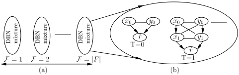
Figure 2 shows a new problem independent DBN mixture, also called value factor mixture, which models Eq. 1. It consists of two mixture variable: F and T. F ranges from 1 to |F|, the total number of value factors. Intuitively, F = i denotes the time dependent DBN mixture for value factor i. A zoomed-in view of the this DBN mixture is provided in Fig. 2(b). The mixture variable F has a fixed, uniform distribution (= 1/|F|). The distribution of the variable T is set as in [Toussaint and Storkey, 2006].
This model relies on the fact that in our representation, each value factor can be represented and evaluated using the DBN mixture of Fig. 2(b) and the reward variable ˆ r as in [Kumar and Zilberstein, 2010]. This DBN mixture for a particular value factor f will contain all the variables for agents involved in factor f : actions, controller nodes and observations, and the state variables Sf . The valuation Vf (Πf ) can be calculated by finding the likelihood L(ˆ r; Πf ) = P(ˆ r = 1; Πf ) of observing ˆ r = 1.
where k and kf are constants, with k being the same for all value factors. This can be easily ensured by making all the original rewards positive by adding a suitable constant. Next we state one of our main results. We will also use a notational convenience that ∑|F | F=1 is equivalent to ∑f∈F .
Theorem 4. Maximizing the likelihood L(ˆ r;Π) of observing ˆ r = 1 in the value factor mixture (Fig.2(a)) is equivalent to optimizing the global policy Π.
Proof. The overall likelihood is given by:
The theorem follows by substituting the value of each L(ˆ r;Πf) in the previous equation from Eq. 2 and the jointpolicy value decomposition assumption of Eq. 1.
3.2 The Expectation-Maximization algorithm
We now derive the EM algorithm for maximizing the likelihood L(ˆ r;Π) in the value factor mixture. Only ˆ r = 1 is observed data, the rest are latent variables. We first handle the infinite horizon case, assuming a stationary policy. Later, we address finite-horizon problems. Note that our derivations differ markedly from [Toussaint and Storkey, 2006] or [Kumar and Zilberstein, 2010] as they focus on a single-agent problem or a 2-agent Dec-POMDP. Our focus is on scalability w.r.t. the number of agents and generality.
An assignment to the mixture variables T and F = f denotes a T-step DBN for the value factor f. For example, assume that the DBN mixture in Fig. 2(b) is for value factor f. Then F = f and T = 1 denote the 1-step DBN (the second DBN) in Fig. 2(b). Let zt denote all the hidden variables for a single time slice t in this DBN. Let Zf = z0...T denote a complete assignment to all the variables from slice 0 to T. We assume for simplicity that each value factor f involves k agents. The full joint for the mixture is:
where the subscript fi denotes the respective parameters for agent i involved in factor f. The square brackets denote dependence upon time: [πfi (a, q)]t = πfi (at = a, qt = q). We also use [P(v, ¯ v)]t to denote P(vt = v, vt-1 = ¯ v). Zf\(Af ,Qf) denotes all the variables in this DBN except the action and controller nodes of all the agents. The structure of this equation is model independent as by conditional independence of policy parameters (π(a, q) = P(a|q)), the first part of the equation (the product terms) can always be written this way. Since EMmaximizes the log-likelihood, we take the log of the above to get:
EMmaximizes the following expected log-likelihood:
where Π denotes the previous iteration's joint-policy and Π⋆ is the current iteration's policy to be determined by maximization. The structure of the log term (Eq. 4) is particularly advantageous as it allows us to perform maximization for each parameter of each agent independently. This does not imply complete problem decoupling as all the parameters still depend on the previous iteration's parameters for all other agents. We first derive the update for the action parameter of an agent j. P(F) can be ignored as it is a constant. Q(Π, Π⋆ ) for action updates is given by:
To maximize this expression, we only need to consider the set of factors f that include agent j, denoted F(j). And because the policy is stationary, Q(Π, Π⋆ ) can be simplified:
Let μj (a, q; Πf ) be defined for each agent j and each factor f ∈ F(j) as follows:
This expression can be easily maximized by using the Lagrange multiplier for the constraint ∑a πj(a, q) = 1. The final update for agent j's action parameters is:
Cq is a normalization constant. The update for λj(p, ¯ p, y) can be found analogously by defining a function μj(p, ¯ p, y; Πf ) along the lines of Eq. 6. The parameter νj can be updated similarly. Therefore the E-step in the EM algorithm involves computing the function μj for each agent j and each factor f ∈ F(j). Eq. 7 specifies the M-step.
Finite-horizon planning
EM can be easily adapted to the finite-horizon case with planning horizon H and no discounting (hence P(T) = 1/H is uniform). Each agent has a non-stationary policy represented as an acyclic FSM. That is, each controller variable qt represents possible controller states at time t. The only difference lies in the definition of the μ functions:
Notice that computing the μ functions is simpler than in the infinite-horizon case (Eq. 6). The above inference requires separate computation in each DBN of length T =t until T = H. The global update rule (Eq. 7) remains the same.
Scalability and message-passing implementation The description of the μ functions highlights the high scalability of EM. Even though the planning problem is highly coupled with each agent, state variables allowed to participate in multiple value factors (see Eq. 1), yet updating policy parameters requires separate local inference in each factor to compute the μ function. The global update rule (Eq. 7) combines such local inferences to provide a monotonic increase in overall solution quality. Each local inference is model dependent and can be computed using standard probabilistic techniques. As our problem setting includes sparse factors, such local inference will be computationally much simpler than performing it on the complete planning model.
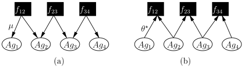
Further, the E and M-steps can be implemented using a parallel, distributed message-passing on a bipartite valuefactor graph G = (U, V,E). The set U contains a node uj for each agent j. The set V contains a node vf for each factor f ∈F. An edge e=(uj, vf) is created if agent j is involved in factor f . Fig. 3 shows such a graph with three value factors in the black squares (the set V ) and 4 agents (the set U).
During the E-step, each factor node vf computes and sends the message μf→j =μj(·;Πf) to each node uj that is connected to vf . Fig. 3(a) shows this step. An agent node uj upon receiving all the μ messages from each factor node connected to it, updates its parameters as in Eq. 7 and sends the updated policy parameters θ⋆ back to each factor node it is connected to (see Fig. 3(b)). This procedure repeats until convergence. Another significant advantage is that all messages can be computed in parallel by each factor node. Our experiments, using an 8-core CPU resulted in near linear speedup over a sequential version. These characteristics of the EM algorithm significantly enhance its scalability for large, but sparse planning problems.
Nature of local optima Variants of the Dec-POMDP model are often solved by fixing the policies of a group of agents and then finding the best response policy of the agent that interacts with the group [Nair et al., 2003; Witwicki and Durfee, 2010]. EM offers significant advantages over such strategy. While both find local optima, EM is more stringent and satisfies the Karush-Kuhn-Tucker conditions [Bertsekas, 1999], which is the norm in nonlinear optimization. The bestresponse strategy provides no such guarantees. Furthermore, in Dec-POMDPs computing the best response is exponential in the plan horizon [Nair et al., 2003]. EM does not suffer this drawback as it directly performs inferences on the DBN.
Dec-MDP, ND-POMDP updates We derived EM updates for infinite-horizon transition-independent Dec-MDPs [Becker et al., 2004] and ND-POMDPs [Nair et al., 2005]. Note that even 2-agent Dec-MDPs are NP-Complete. To the best of our knowledge, no algorithm can scale up to more than two agents for these models (with infinite-horizon). This underscores the practical significance of EM. Eqs. 9-10 show the μ functions for Dec-MDPs and ND-POMDPs. u denotes the internal state of an agent; the rest of the notation is as in [Kumar and Zilberstein, 2010]. Other parameters can be updated similarly, not listed due to space reasons. Computing the μ functions is polynomial in all problem parameters.
4 Experiments
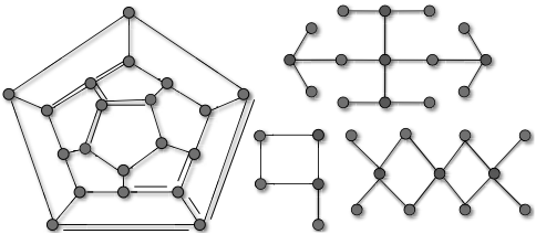
We experimented on a target tracking application in sensor networks modeled as an ND-POMDP [Nair et al., 2005]. Fig. 4 shows four sensor topologies: 5P, 11H and 15-3D from [Marecki et al., 2008] and the largest 20D from [Kumar and Zilberstein, 2009]. Each node in these graphs is a sensor agent and edges are locations where targets can move. Tracking a target requires simultaneous scan of the edge by two adjacent sensors, producing a joint reward (+80), otherwise a penalty (-1) is given per scanning agent. The internal state of a sensor indicates its battery level (5 possible states). Each scan action depletes the battery and an empty battery renders the sensor unusable. Sensors can conserve power with the off action or recharge the battery at some cost (-1). Each sensor has three observations: target present, target absent and idle. The first two observations can be false positive/negative. EM was implemented in JAVA. All the experiments used an 8-core Mac Pro with 2GB RAM, using multithreading to utilize all 8-cores. Each plot is the best of 10 runs. The discount factor γ was 0.95. To speed up EM's convergence, we used a greedy variant of the M-step [Toussaint et al., 2008].
The 5P domain has 2 targets, 11H has 3 targets, 15-3D has 5 targets, and 20D has 6 targets. These problems have very large state-spaces: 6 × 55 for 5P, 64 × 511 for 11H, 144×515 for 15-3D and 2700×520 for 20D. Evidently, EM efficiently exploits the factored representation of the state and action spaces and is highly scalable with linear complexity w.r.t. the number of edges in the graph.
Figure 5 shows the solution quality EM achieves for each of these benchmarks with different controller sizes. A notable observation from these graphs is that EM converges quickly, taking fewer than 200 iterations even for such large multiagent planning problems. The solution quality, as expected, increases monotonically with each iteration highlighting the anytime property of EM. In general, the solution quality increased with the number of controller nodes. For example, for 20D, a 2-node controller achieves a quality of 3585.06
| Instance\Size | 2-Node | 3-Node | 4-Node | 5-Node |
|---|---|---|---|---|
| 5P | .232 | 1.07 | 3.22 | 7.74 |
| 11H | 1.29 | 6.07 | 18.90 | 45.23 |
| 15-3D | 1.17 | 5.39 | 16.69 | 40.47 |
| 20D | 5.03 | 22.01 | 67.85 | 171.26 |

| Instance/Value | EM | U.B. | Random |
|---|---|---|---|
| 5P | 1250.89 (44.3%) | 2820 | 61.23 |
| 11H | 1509.27 (35.6%) | 4230 | 8.41 |
| 15-3D | 3094.05 (43.8%) | 7050 | 104.2 |
| 20D | 4154.04 (49.1%) | 8460 | -31.67 |
| Internal State = 2 | Internal State = 3 | |||
|---|---|---|---|---|
| N | EM | NLP | EM | NLP |
| 2 | 670.8/3.8 | 79/5.4 | 972.5/8.9 | 905.7/17.8 |
| 3 | 670.8/13.02 | 140.4/14.5 | 1053.16/35.8 | 887.2/139 |
| 4 | 710.4/35.8 | 140.4/139.4 | 1062.4/107.4 | 1024.8/1078.1 |
and a 5 node controller achieves 4154.04. However, for 5P and 15-3D, we did not observe a significant increase in quality by increasing controller size, possibly due to the relative simplicity of these configurations.
Table 1 shows the runtime per iteration of EM for different instances and varying controller sizes. Encouragingly, the runtime is fairly small-particularly for smaller controller sizes-even for large problems such as 20D. To further decrease the runtime for larger controllers, we plan to use Monte-Carlo sampling techniques in the future.
Table 2(a) shows the solution quality comparison of EM with random controllers and a loose upper bound. The upper bound was computed by assuming that each target is detected at every time step including the battery recharge cost. Against random controllers, EM always achieves much better solution quality. When compared against the upper bound, we can see that EM performs quite well. Despite being a very loose bound, EM still achieves a quality within 49.1% of this bound for the largest 20D domain-a solid performance.
Currently no algorithm can solve infinite-horizon NDPOMDPs (>2-agents). To further assess EM's performance, we developed a nonlinear programming (NLP) formulation of the problem and used a state-of-the-art NLP solver called Snopt [Gill et al., 2002]. Snopt could only solve the smallest 5P domain and could not scale beyond controller size 4 and internal state 3 as it ran out of memory (=2GB). Table 2(b) shows the solution quality and time comparisons. For internal state size of 2, Snopt gets stuck in a poor local optimum compared to EM. It provides more competitive solutions for internal state 3, but EM is still better in solution quality. Furthermore, the runtime of Snopt degrades quickly with the increase in nonlinear constraints. This makes Snopt about an order-of-magnitude slower for controller size 4 and internal state 3. These results further highlight the scalability of EM, which could scale up to controller size 10 and internal state 5 within 2GB RAM and ≈ 4 hours for 100 iterations.
Table 3 shows a comparison of EM against handcrafted controllers designed to take into account the target trajectories and partial observation in the 11H benchmark (Fig. 4). To simplify the problem for the handcrafted solution, all penalties were zero and the reward for detecting a target was 1. This allowed continuous scan by sensors without worrying about miscoordination penalty. The first row in this table shows this no penalty case. We see that EM is competitive with the handcrafted controller. The second row shows the results when there was a cost to charge batteries. In this case, sensors need to decide when to become idle to conserve power. The handcrafted controller cannot learn this behavior and hence EM produces much better quality in this case.
| Version \ FSC Size | Handcrafted | 2 (EM) | 3 (EM) | 4 (EM) |
| No penalty | 13.92 | 13.95 | 15.48 | 15.7 |
|---|---|---|---|---|
| Penalty (-.25) | -3.36 | 5.27 | 5.27 | 5.27 |
Finally, Table 4 highlights the significant opportunities that EM provides for parallel computation. We consistently obtained almost linear speedup when using multithreading on an 8-core CPU (total possible parallel threads in the largest domain 20D is 60). By using a massively parallel platform such a Google's MapReduce,we could easily solve much larger team decision problems than currently possible.
5 Conclusion
Despite the rapid progress in multiagent planning, the scalability of the prevailing formal models has been limited. We present a new approach to multiagent planning by identifying the general property of value factorization that facilitates the development of a scalable approximate algorithm using probabilistic inference. We show that several existing classes of Dec-POMDPs satisfy this property. In contrast to previous approaches, our framework does not impose any further restrictions on agent interaction beyond this property, thus providing a general solution for structured multiagent planning.
| Version \ FSC Size | 2 | 3 | 4 | 5 |
|---|---|---|---|---|
| Serial | 41.05 | 177.54 | 543.52 | 1308.20 |
| Parallel | 5.03 | 22.01 | 67.85 | 171.26 |
The key result that supports the scalability of our approach is that, within the EM framework, the inference process can be decomposed into separate components that are much smaller than the complete model, thus avoiding an exponential complexity. Additionally, the EM algorithm allows for distributed planning using message-passing along the edges of the value-factor graph, and is amenable to parallelization. It also provides significant advantages over existing locally optimal approaches for Dec-POMDPs, delivering more rigorous guarantees on the solution. Results on large sensor network problems confirm the scalability of our approach.
Our approach offers a form of policy iteration using finitestate controllers to represent policies; extending it to the value iteration is an important future work. We currently assume that the structure of each value factor remains static. A significant contribution would be to allow agents to change this structure via their actions and still provide the current guarantees. Overall, this new approach promises to significantly enhance the scalability and practical applicability of decentralized POMDPs.
Acknowledgments
We thank the anonymous reviewers for helpful suggestions. This work was funded in part by the National Science Foundation under grant IIS-0812149, the Air Force Office of Scientific Research under grant FA9550-08-1-0181 and the German Research Foundation (DFG), Emmy Noether fellowship TO 409/1-3.
@inproceedings{ijcai2011p357,
  title     = {Scalable Multiagent Planning Using Probabilistic Inference},
  author    = {Kumar, Akshat and Zilberstein, Shlomo and Toussaint, Marc},
  booktitle = {Proceedings of the Twenty-Second International Joint Conference on
               Artificial Intelligence, {IJCAI-11}},
  publisher = {AAAI Press/International Joint Conferences on Artificial Intelligence},
  editor    = {Toby Walsh},
  pages     = {2140--2145},
  year      = {2011},
  month     = {7},
  doi       = {10.5591/978-1-57735-516-8/IJCAI11-357},
  url       = {https://doi.org/10.5591/978-1-57735-516-8/IJCAI11-357},
}
TY - CPAPER TI - Scalable Multiagent Planning Using Probabilistic Inference AU - Kumar, Akshat AU - Zilberstein, Shlomo AU - Toussaint, Marc T2 - Proceedings of the Twenty-Second International Joint Conference on Artificial Intelligence, IJCAI-11 PB - AAAI Press/International Joint Conferences on Artificial Intelligence PY - 2011 SP - 2140 EP - 2145 DO - 10.5591/978-1-57735-516-8/IJCAI11-357 UR - https://doi.org/10.5591/978-1-57735-516-8/IJCAI11-357 ER -Copied
Machine-readable versions of this paper, for tools and AI agents:





