
Existential arc consistency: Getting closer to full arc consistency in weighted CSPs
Proceedings of the Nineteenth International Joint Conference on Artificial Intelligence. Pages 84-88.
© 2005 International Joint Conferences on Artificial Intelligence
Abstract
The weighted CSP framework is a soft constraint framework with a wide range of applications. Most current state-of-the-art complete solvers can be described as a basic depth-first branch and bound search that maintain some form of arc consistency during the search. In this paper we introduce a new stronger form of arc consistency, that we call existential directional arc consistency and we provide an algorithm to enforce it. The efficiency of the algorithm is empirically demonstrated in a variety of domains.
- [Bessiere and Regin, 2001] C. Bessiere and J.C. Regin. Re- fining the basic constraint propagation algorithm. In IJCAI-01, pages 309-315, 2001. IJCAI
- [Cooper and Schiex, 2004] M. Cooper and T. Schiex. Arc consistency for soft constraints. Artificial Intelligence, 154:199-227, 2004.
- [Erlenkotter, 1978] D. Erlenkotter. A Dual-Based Procedure for Uncapacitated Facility Location. Operations Research, 26(6):992-1009, 1978.
- [Körkel, 1989] M. Körkel. On the exact solution of large- scale simple plant location problems. European Journal of Operational Research, 39:157-173, 1989.
- [Kratica et al., 2001] J. Kratica, D. Tosic, V. Filipovic, and I. Ljubic. Solving the Simple Plant Location Problems by Genetic Algorithm. RAIRO Operations Research, 35:127- 142, 2001.
- [Larrosa and Schiex, 2003] J. Larrosa and T. Schiex. In the quest of the best form of local consistency for weighted CSP. In IJCAI-03, pages 239-244, 2003. IJCAI
- [Larrosa and Schiex, 2004] J. Larrosa and T. Schiex. Solving Weighted CSP by Maintaining Arc-consistency. Artificial Intelligence, 159(1-2):1-26, 2004.
- [Michel and Hentenryck, 2004] L. Michel and P. Van Hen- tenryck. A Simple Tabu Search for Warehouse Location. European Journal on Operations Research, 157(3):576- 591, 2004.
- [Schiex et al., 1995] T. Schiex, H. Fargier, and G. Verfail- lie. Valued constraint satisfaction problems: hard and easy problems. In IJCAI-95, pages 631-637, 1995. IJCAI
References were extracted automatically from the PDF and may contain errors.
Full text extracted automatically from the PDF; figures, tables and equations may differ. The PDF is the version of record.
1 Introduction
Weighted constraint satisfaction problems (WCSP) is a wellknown optimization version of the CSP framework with many practical applications. Recently, the celebrated arc consistency property has been generalized from the classical CSP framework to WCSP [Cooper and Schiex, 2004; Larrosa and Schiex, 2004]. There are three known generalizations: AC*, FDAC* and FAC*, all of them collapsing to classical arc consistency in the CSP case. In [Larrosa and Schiex, 2003] it was shown that maintaining FDAC* during search was usually the best option.
In this paper we introduce a new form of local consistency called existential directional arc consistency (EDAC*). We show that EDAC* is stronger than FDAC* and we introduce an algorithm to enforce EDAC* that runs in time O(ed 2 ×max{nd,⊤}), where e, n and d are the number of constraints, variables and domain values, respectively; ⊤ is the upper bound of the WCSP instance (to be defined later). The main use of EDAC* and its associated filtering algorithm is to embed it into a complete depth-first branch and bound solver that maintains EDAC* at every visited node. We have experimentally evaluated this idea on randomMaxSAT, Max-CSP, and uncapacitated warehouse location problems. We observe that maintaining EDAC* is never worse than maintaining FDAC* and, in many instances, it is orders of magnitude better.
∗This research is partially supported by the French-Spanish collaboration PICASSO 05158SM - Integrated Action HF02-69 and the REPLI project TIC-2002-04470-C03.
Federico Heras fheras@lsi.upc.edu Javier Larrosa larrosa@lsi.upc.edu LSI, UPC Barcelona, Spain
2 Preliminaries
Valuation structures are algebraic objects to specify costs in valued constraint satisfaction problems [Schiex et al., 1995]. They are defined by a triple S = (E,⊕,⪰), where E is the set of costs totally ordered by ⪰. The maximum and a minimum costs are noted ⊤ and ⊥, respectively. ⊕ is an operation on E used to combine costs.
Following [Larrosa and Schiex, 2004], the valuation structure of Weighted CSP (WCSP) is, S(k) = ([0..k],⊕,≥) where k > 0 is a natural number; ⊕ is defined as a⊕b = min{k, a+ b}; ≥ is the standard order among naturals. Observe that in S(k), we have 0 = ⊥ and k = ⊤. It is useful to define the subtraction ⊖ of costs. Let a, b ∈ [0..k] be two costs such that a ≥ b,
A binary weighted constraint satisfaction problem (WCSP) is a tuple P= (S(k),X ,D,C). S(k) is the valuation structure. X = {x1, . . . ,xn} is a set of variables that we will often call by just their index. Each variable xi ∈ X has a finite domain Di ∈D of values that can be assigned to it. (i,a) denotes the assignment of value a ∈Di to variable xi. C is a set of unary and binary weighted constraints (namely, cost functions) over the valuation structure S(k). A unary weighted constraint Ci is a cost function Ci(xi) → [0..k]. A binary constraint Ci j is a cost function Ci j(xi,xj) → [0..k] We assume the existence of a unary constraint Ci for every variable, and a zero-arity constraint (i.e. a constant), noted C∅ (if no such constraint is defined, we can always define dummy ones: Ci(xi) = ⊥, C∅ = ⊥).
When a constraint C assigns cost ⊤, it means that C forbids the corresponding assignment, otherwise it is permitted by C with the corresponding cost. The cost of an assignment X = (x1, . . . , xn), noted V (X), is the sum over all the problem cost functions,
An assignment X is consistent if V(X) < ⊤. The usual task of interest is to find a consistent assignment with minimum cost, which is NP-hard. Observe that WCSP with k = 1 reduces to classical CSP.
Algorithm 1: Algorithms to propagate costs.
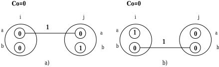
Function PruneVar(i) : boolean f lag := false ; foreach a ∈ Di do if (C∅⊕Ci(a) ≥⊤) then Di :=Di -{a} ; f lag := true ; return f lag ; Procedure ProjectUnary(i) a := mina∈Di {Ci(a)} ; C∅ :=C∅⊕a ; foreach a ∈ Di do Ci(a) :=Ci(a)⊖a ; Procedure Project(i,a, j,a) Ci(a) :=Ci(a)⊕a ; foreach b ∈Dj doCi j(a,b) :=Ci j(a,b)⊖a ; Procedure Extend(i,a, j,a) foreach b ∈Dj doCi j(a,b) :=Ci j(a,b)⊕a ; Ci(a) :=Ci(a)⊖a ;Example 1 Consider the problem depicted in Figure1.a. It has two variables i, j with two values (a,b) in their domains. Unary costs are depicted within small circles. Binary costs are represented by edges connecting the corresponding values. The label of each edge is the corresponding cost. If two values are not connected, the binary cost between them is 0. In this problem the optimal cost is 0 and it is attained with the assignment (b,a).
3 Some local consistencies inWCSP
Two WCSPs defined over the same variables are said to be equivalent if they define the same cost distribution on complete assignments. Local consistency properties are widely used to transform problems into equivalent simpler ones. In general, constraints can be given explicitly as tables of costs, or implicitly as mathematical expressions or algorithmic procedures. For simplicity in our exposition, we will assume the explicit form. This is done without loss of generality as discussed in [Cooper and Schiex, 2004]. The simplest form of local consistency is Node consistency (NC*).
Definition 1 Variable xi is node consistent if: for all values a ∈ Di, C∅ ⊕Ci(a) < ⊤ , and there exists a value a ∈ Di such that Ci(a) =⊥. A WCSP is node consistent (NC*) if every variable is node consistent.
Any WCSP can be easily transformed into an equivalent NC* instance by projecting every unary constraints towards C∅ and subsequently pruning every unfeasible value. Functions ProjectUnary and PruneVar (Algorithm1) perform the projection of a unary constraint towards C∅ and prune unfeasible values, respectively.
Arc consistency properties are based on the notion of simple and full support. Given a binary constraint Ci j, we say that b ∈ Dj is a simple support for a ∈ Di if Ci j(a,b) = ⊥. Similarly, we say that b ∈ Dj is a full support for a ∈ Di if Ci j (a, b) ⊕C j (b) = ⊥.
Definition 2 Variable xi is arc consistent if every value a ∈ Di has a simple support in every constraint Ci j. A WCSP is arc consistent (AC*) if every variable is node and arc consistent.
Definition 3 Variable xi is full arc consistent if every value a ∈ Di has a full support in every constraint Ci j . A WCSP is full arc consistent (FAC*) if every variable is node and full arc consistent.
Simple supports for a ∈ Di in Dj can be enforced by projecting binary costs Ci j(a, ·) towards Ci(a), as performed by procedure Project (Algorithm 1). Procedure FindSupports (Algorithm 2) enforces simple supports in Dj for every value in Di .
Example 2 The WCSP depicted in Figure2.a is not AC* because value a ∈ Di does not have a simple support in variable j. AC* is enforced by executing FindSupports(i, j) (producing the problem in 2.b) and then ProjectUnary(i) (producing the problem in 2.c).
To enforce full supports for Di values in Dj (Procedure FindFullSupports in Algorithm 2) we need to extend unary costs fromCj (·) towards Ci j (·, ·) (procedure Extend in Algorithm 1). Then, binary costs are projected towards Ci(a).
In the CSP case (i.e, k = 1), being a simple support for (i, a) is equivalent to being a full support for it and both notions reduce to the classical notion of support. Therefore, AC* and FAC* reduce to classical arc consistency. In the WCSP case, however, being a full support is stronger than being a simple support. In [Larrosa and Schiex, 2004] it was shown that every WCSP can be transformed into an equivalent arc consistent one in time O(ed 3 ). Unfortunately, not every WCSP can be transformed into an equivalent full arc consistent one.
Example 3 The problem in Figure1.a is AC*, but it is not FAC* because value a∈Di is not fully supported. We can enforce the full support by calling FindFullSupports(i, j). The resulting problem, depicted in Figure1.b is not FAC* because value b ∈ Dj is not fully supported. If we enforce the full support by calling FindFullSupports( j, i), we return to the problem in Figure1.a. It can be easily proved that this problem does not have an equivalent FAC* one.
Therefore, FAC* is not a practical property. To circumvent this problem, a weaker property has been proposed. In the sequel, we assume that the set of variables X is totally ordered by >.
Definition 4 Variable xi is directional arc consistent if every value a ∈ Di has a full support in every constraint Ci j such
Algorithm 2: Algorithms to enforce supports. Function FindSupports(i, j) : boolean f lag := false ; foreach a ∈ Di do a :=minb∈Dj {Ci j(a,b)} ; if (a>⊥∧Ci(a) =⊥) then f lag := true ; Project(i,a, j,a) ; ProjectUnary(i) ; return f lag ; Function FindFullSupports(i, j) : boolean f lag := false ; foreach a ∈ Di do P[a] :=minb∈Dj {Ci j(a,b)⊕Cj(b)} ; if (P[a] >⊥∧Ci(a) =⊥) then f lag := true ; foreach b ∈ Dj do E[b] :=maxa∈Di {P[a]⊖Ci j(a,b)} ; foreach b ∈ D j do Extend( j, b, i,E[b]) ; foreach a ∈ Di do Project(i,a, j,P[a]) ; ProjectUnary(i) ; return f lag ; Function FindExistentialSupport(i) : boolean f lag := false ; 1 a :=mina∈Di {Ci(a) ⊕Ci j∈C s.t. j<i minb∈Dj {Ci j(a,b)⊕Cj(b)}}; if (a>⊥) then 2 foreachCi j ∈C s.t. j < i do f lag := f lag ∨ FindFullSupports(i, j) ; return f lag ;that j > i. It is full directional arc consistent (FDAC) if, in addition, every value a ∈ Di has a simple support in every constraint Ci j such that j < i. A WCSP is full directional arc consistent (FDAC*) if every variable is node and full directional arc consistent.
Example 4 The problem in 2.c is AC* but not FDAC*, because value a ∈ i does not have a full support in variable j. FDAC* is enforced by executing FindFullSupports(i, j) (producing the problem in Figure 2.d).
Every WCSP can be transformed into an equivalent FDAC* WCSP with time complexity O(end 3) [Larrosa and Schiex, 2003]. In the CSP case, FDAC* also reduces to classical arc-consistency. In the general case FAC* implies FDAC* and FDAC* implies AC* (namely, the satisfaction of one property implies the satisfaction of the other). An important question is whether it is possible to strengthen the FDAC* property to make it closer to FAC*, but still having the guarantee of existence for an arbitraryWCSP instance. In the next Section we address this issue.
4 Existential arc consistency: a stronger new property
Consider the FDAC* problem in Figure2.d. Observe that value a ∈ Dk has a simple support in x j (required by the FDAC* property) but does not have any full support. We have the same situation with value b ∈ Dk and variable xi.
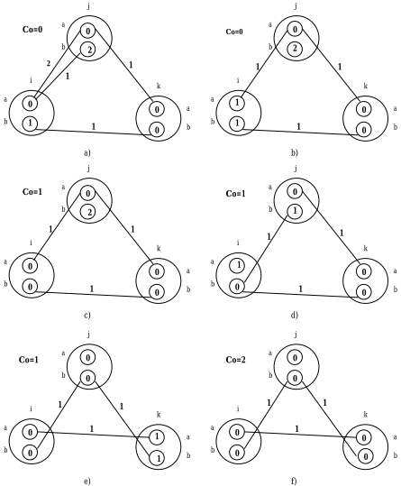
As a consequence, the unary cost of both values in Dk can be increased by enforcing full supports (Figure 2.e). Since all unary costs of Di values are larger than zero, node consistency is lost and the lower bound can be increased (Figure 2. f ). In general, full supports can be safely enforced in both directions if their enforcement produces an increment in the lower bound. Next, we show that there is a natural local consistency property behind this observation, that we call existential arc consistency (EAC*).
Definition 5 Variable xi is existential arc consistent if there is at least one value a ∈ Di such that Ci(a) =⊥ and it has a full support in every constraint Ci j . A WCSP is existential arc consistent (EAC*) if every variable is node and existential arc consistent.
All the previous forms of arc consistency required the same condition for every domain value. However, EAC* requires the existence for every variable of a special value. The important fact to note is: if a variable xi is not EAC*, then for all domain value a with Ci(a) = ⊥ there is a variable x j such that ∀b ∈ Dj,Ci j(a,b)⊕Cj(b) >⊥. Thus enforcing full supports in xi will break the NC* property and it will be possible to increase the lower bound. It is possible to integrate EAC* with FDAC* in order to exploit the benefits of each. It is achieved by the existential directional arc consistency (EDAC*) property.
Definition 6 A WCSP is EDAC* if it is FDAC* and EAC*.
In words, EDAC* requires that every value is fully supported in one direction and simply supported in the other direction (to satisfy FDAC*). Additionally, at least one value per variable must be fully supported in both directions (to satisfy EAC*). The special value is called the fully supported value. Observe that in the CSP case EDAC* instantiates to classical arc consistency. Besides, EDAC* is weaker than FAC*, but stronger than FDAC*.
5 Algorithm
We present an algorithm for the enforcement of EDAC* in the case of binary WCSPs. EDAC* (Algorithm 3) transforms an arbitrary problem into an equivalent one verifying the EDAC* local property. It uses three propagation queues, Q, R and P, that are implemented as priority queues so that the lowest or the highest variable in the queue can be popped in constant time. If j ∈ Q, it means that some value in Dj has been pruned (neighbors of j higher than j may have lost their simple support and must be revised). If j ∈ R, it means that some value in Dj has increased its unary cost from ⊥ (neighbors of j lower than j may have lost their full support and must be revised). If i ∈ P, it means that some value in Dj ( j < i neighbor of i) has increased its unary cost from⊥ (i may have lost the full support of its fully supported value and must be revised). Besides, there is an auxiliary queue S that is used to efficiently build P.
The algorithm is formed by a main loop, with four inner loops. The while loops at lines 5, 8 and 10 respectively enforce EAC*, DAC* and AC*; the line 11 enforces NC*. Each time some costs are projected by the enforcement of a local property, another property may be broken. The variables for which the local property may be broken are stored in a queue for revision. The enforcement of NC*, AC* and DAC* is achieved as proposed in [Larrosa and Schiex, 2003]. Thus, we focus on the enforcement of EAC*.
EAC* enforcement is mainly encoded by Function FindExistentialSupport(i), which enforces the existential support in xi by finding full supports wrt. every lower neighbor xj (it does not have to worry for higher neighbors because DAC* enforcement takes care of them). While enforcing the existential support in xi, the cost functionCj decreases or remains the same. As a consequence, we do not need to revise the existential consistency of x j nor the directional arc consistencies of the lowest neighbors of x j. Furthermore, as the existential consistency is stronger than the arc one, enforcing AC* between xi and xj is useless. However, the directional arc consistency of variable xi should be checked, because some unary cost of xi could have been increased (line 6). Similarly, the existential consistency of higher neighbors of xi should also be verified (line 7).
PruneVar() enforces node consistency after unary cost and lower bound increments (line 11). This function can be executed more often in order to avoid unnecessary value examinations during the while loops. It does not change the worstcase time complexity. For simplicity reasons, the case of inconsistent problems where C∅ reaches ⊤ is not described.
Theorem 1 The complexity of EDAC* is time O(ed 2 max{nd,⊤}) and space O(ed).
Algorithm 3: Enforcing EDAC*, initially, Q=R=S=X .
4
6
7
9
11
Procedure EDAC* 3 while (Q ̸=∅∨R ̸=∅∨S ̸=∅) do P := {l | i ∈ S, l > i,Cil ∈ C}∪S ; S :=∅ ; 5 while (P ̸=∅) do i :=popMin(P) ; if FindExistentialSupport(i) then R :=R∪{i} ; foreachCi j ∈C s.t. j > i do P :=P∪{ j} ; 8 while (R ̸=∅) do j :=popMax(R) ; foreachCi j ∈C s.t. i < j do if FindFullSupports(i, j) then R :=R∪{i} ; S :=S∪{i} ; 10 while (Q ̸=∅) do j :=popMin(Q) ; foreachCi j ∈C s.t. i > j do if FindSupports(i, j) then R :=R∪{i} ; S :=S∪{i} ; foreach i ∈ X do if PruneVar(i) then Q := Q∪{i} ;proof 1 Regarding space, we use the structure suggested by [Cooper and Schiex, 2004] to bring the space complexity to O(ed). [Larrosa and Schiex, 2003] proved that ProjectUnary, Project, Extend and PruneVar are time O(d); FindSupports and FindFullSupports are time O(d 2 ). Let us now focus on the while loop complexities in EDAC*. The loop at line 8 enforces DAC*. As described in previous papers, it is time O(ed 2 ) because each variable is pushed in R at most once and thus each constraint Ci j is checked once (line 9). Similarly, the loop at line 10 which enforces AC*, directed from the lowest variables to the highest ones, is also O(ed 2 ).
The loop at line 5 enforces EAC* directed to the highest variables. In a single run of this loop, a variable will never be pushed twice in P because the popped variable xi is always the lowest one, and the pushed variables are higher than xi. It implies that the while loop iterates at most n times, leading to a O(e) time complexity for line 7. The amortized complexity time of FindExistentialSupport is O(ed 2 ) because this function may be called with each variable, so every binary constraint at line 1 and 2 is observed once. Thus, the time complexity of EAC* is also O(ed 2 ).
The line 4 is time O(n). The for at line 11 is time O(nd) (which is less than O(ed), as the graph is supposed to be connected). Compiling the different results, the complexity inside the while at line 3 is O(ed 2). It loops when:
- either Q is not empty: the for at line 11 has pruned a value and this is done at most nd times;
- either R is not empty: AC* has enqueued a variable in R and by the preceding remark this cannot be done more than O(nd) times;
- or S is not empty: an element has been enqueued while enforcing AC* or DAC*. The first case cannot happen more than O(nd). The second case happens O(max{nd,⊤}) times because the condition at line 8 is true when AC* has added an element in R (O(nd) times) or EAC* has added an element (O(⊤) times because each time EAC* is violated, C∅ increases).
Consequently, the overall complexity is O(ed 2 max{nd,⊤}).
6 Experimental results
In this Section, we perform an empirical comparison of EDAC* with FDAC* for the task of proving optimality. The main use of the EDAC* and FDAC* properties is to use them inside a depth-first branch and bound solver. The idea is to maintain EDAC* and FDAC* during the search (algorithms called MEDAC* and MFDAC*, respectively). We have implemented (C code) this idea in an efficient incremental version that uses tables of supports `a la AC2001 [Bessiere and Regin, 2001]. In non-binary problems, we delay the propagation of non-binary constraints until they become binary. For variable selection we use the dom/deg heuristics which selects the variable with the smallest ratio of domain size divided by future degree. For value selection we consider values in increasing order of unary cost Ci. The variable ordering for directional arc consistency is given by their index. The optimum of each problem instance (except for MAX-SAT where only a good upper bound is provided) is given to the branch and bound as a first upper bound. We experimented with three domains easily modeled as WCSP. Given a CNF formula, Max-SAT is the problem of finding a complete assignment with a maximum number of satisfied clauses. We have generated and solved 80-variable 2-SAT and 40-variable 3SAT instances with varying the number of clauses using Cnfgen 1 , a random k-SAT generator. Note that this generator prevents duplicate or opposite literals in clauses but not duplicate clauses. Given an overconstrained CSP, Max-CSP is the problem of finding a complete assignment with a maximum number of satisfied constraints. We have generated 6 classes of binary random problems with domain size set to 10 (Sparse-Loose (constraint graph connectivity of 12% for 40 variables), Sparse-Tight, Dense-Loose (constraint graph connectivity of 25%), Dense-Tight, Complete-Loose, and Complete-Tight) as proposed in [Larrosa and Schiex, 2003]. In Max-SAT (resp. Max-CSP), samples have 10 (resp. 50) instances and we report mean values. In the uncapacitated warehouse location problem (UWLP) a company considers opening warehouses at some candidate locations in order to supply its existing stores. The objective is to determine which warehouses to open, and which of these warehouses should supply the various stores, such that the sum of the maintenance and supply costs is minimized. Each store must be supplied by exactly one open warehouse. We simply model the problem by l boolean variables for the candidate locations, s integer variables for the stores with domain size set to l, l +s soft unary constraints for the costs, and l ×s hard binary constraints connecting stores and warehouses. We took and solved the problem instances cap71-134 from the standard OR Library benchmarks for UWLP, as well as the MO*- MP* instances by courtesy of J. Kratica [Kratica et al., 2001]. The M* instances are very challenging for mathematical programming approaches because they have a large number of suboptimal solutions.
1 A. van Gelder ftp://dimacs.rutgers.edu/pub/challenge/ satisfiability/contributed/UCSC/instances
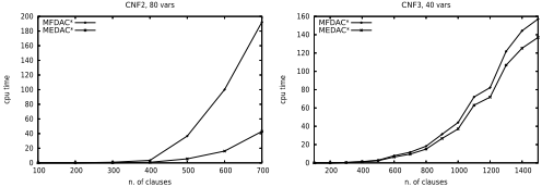
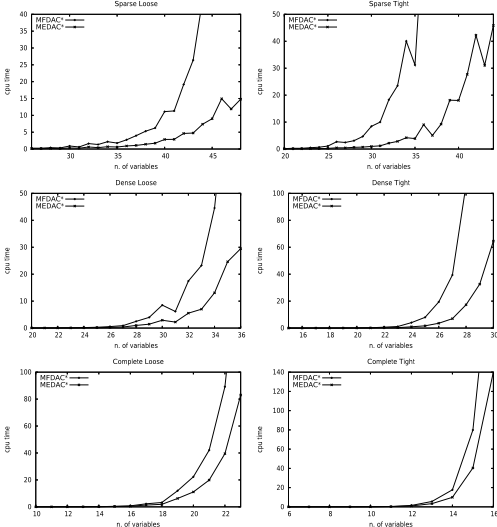
The experiments were all performed on a 2.0 GHz Pentium 4 computer with 512 MB 2 . Time results in seconds are given in Figures 3 and 4, and Table 5. In all Max-SAT (resp. Max-CSP classes), the search effort seems to grow exponentially with the number of clauses (resp. number of variables). We summed the computation times for all the samples that were completely solved by both algorithms and computed the ratio MFDAC*/MEDAC* . In Max-2SAT, MEDAC* was 5.1 faster than MFDAC*. The improvement is lower in Max-3SAT. We think this result is due to our simple delaying mechanism for tackling n-ary constraints. For MaxCSP, MEDAC* was faster than MFDAC* by a factor ranging from 2.0 (Complete-Tight) to 9.52 (Sparse-Tight). The same results were observed when analyzing the number of nodes expanded by MEDAC* and MFDAC* (not reported here for lack of space). In summary, the speed-up obtained was even more important on problems with small constraint graph connectivity.
2 The program named TOOLBAR and the benchmarks are available at http://carlit.toulouse.inra.fr/cgi-bin/ awki.cgi/SoftCSP.
| Problem | Size | MFDAC∗ | MEDAC∗ | CPLEX |
|---|---|---|---|---|
| cap71 | 16 × 50 | 0.01 | 0.00 | 0.02 |
| cap72 | 16 × 50 | 0.01 | 0.01 | 0.00 |
| cap73 | 16 × 50 | 0.02 | 0.01 | 0.00 |
| cap74 | 16 × 50 | 0.02 | 0.01 | 0.02 |
| cap101 | 25 × 50 | 0.03 | 0.02 | 0.02 |
| cap102 | 25 × 50 | 0.13 | 0.03 | 0.01 |
| cap103 | 25 × 50 | 0.35 | 0.03 | 0.01 |
| cap104 | 25 × 50 | 0.24 | 0.04 | 0.01 |
| cap131 | 50 × 50 | 65.02 | 0.11 | 0.05 |
| cap132 | 50 × 50 | 155.08 | 0.12 | 0.04 |
| cap133 | 50 × 50 | 194.36 | 0.14 | 0.05 |
| cap134 | 50 × 50 | 44.75 | 0.12 | 0.05 |
| MO1 | 100 × 100 | - | 216.57 | 202.48 |
| MO2 | 100×100 | 11775.60 | 44.45 | 36.67 |
| MO3 | 100×100 | 15123.70 | 74.60 | 199.84 |
| MO4 | 100×100 | 3525.61 | 31.74 | 43.26 |
| MO5 | 100×100 | 2354.95 | 33.98 | 42.96 |
| MP1 | 200 × 200 | - | 3403.37 | 2296.65 |
| MP2 | 200 × 200 | - | 1443.93 | 917.92 |
| MP3 | 200 × 200 | - | 981.28 | 1209.15 |
| MP4 | 200 × 200 | - | 1768.51 | 1936.57 |
| MP5 | 200 × 200 | - | 1099.88 | 697.51 |
For UWLP, MEDAC* is several orders of magnitude faster than MFDAC* for problem size l ≥ 50. We concluded that the lower bound computed by EDAC* for UWLP is stronger and less variable ordering dependent than the FDAC* one. Although UWLP is well-solved by dedicated mathematical programming approaches [Erlenkotter, 1978; K¨orkel, 1989] and heuristic search methods [Kratica et al., 2001; Michel and Hentenryck, 2004], it is worth noticing that our generic WCSP algorithm was able to solve to optimality moderatelysized problems in reasonable time (in less than 1 hour). For comparison purposes, we solved UWLP instances using a state-of-the-art mixed-integer programming solver Ilog CPLEX 9.0 with default parameters (and without initial upper bounds) and a direct formulation of the problem. MEDAC* and CPLEX obtained results within the same order of magnitude in terms of cpu time.
Reversing the order of lines 5 (EAC* loop), 8 (DAC* loop), and 10 (AC* loop) in MEDAC* slowed down the algorithm by a factor 3 2 on our Max-CSP benchmarks. It is important to increase the lower bound as soon as possible as it is done first by EAC*. We are currently investigating a lazy implementation of EAC* where the constraints in line 2 are projected only for the purpose of increasing the lower bound and not for pruning the values. This allows to reduce the number of variables inserted in R and P by EAC* and, consequently, the number of iterations of the different loops.
7 Conclusions and future work
In this paper we have introduced a new local consistency property called EDAC* and adapted it to WCSP. We have studied its complexity, and despite its theoretical cost, it has been shown that maintaining EDAC* is always better than maintaining FDAC* in a variety of domains. In the future, we want to study a lazy version of EDAC* and to apply it to other problems.
Acknowledgments
The authors are grateful to Thomas Schiex for useful comments on an early version of the paper and to Julia Larrosa for being born after the submission deadline.
@inproceedings{ijcai2005p90,
  title     = {Existential arc consistency: Getting closer to full arc consistency in weighted CSPs},
  author    = {de Givry, Simon and Heras, Federico and Zytnicki, Matthias and Larrosa, Javier},
  booktitle = {Proceedings of the Nineteenth International Joint Conference on
               Artificial Intelligence, {IJCAI-05}},
  publisher = {International Joint Conferences on Artificial Intelligence},
  editor    = {Leslie Pack Kaelbling and Alessandro Saffiotti},
  pages     = {84--88},
  year      = {2005},
  url       = {https://ijcai.org/proceedings/2005/90},
}
TY - CPAPER TI - Existential arc consistency: Getting closer to full arc consistency in weighted CSPs AU - de Givry, Simon AU - Heras, Federico AU - Zytnicki, Matthias AU - Larrosa, Javier T2 - Proceedings of the Nineteenth International Joint Conference on Artificial Intelligence, IJCAI-05 PB - International Joint Conferences on Artificial Intelligence PY - 2005 SP - 84 EP - 88 UR - https://ijcai.org/proceedings/2005/90 ER -Copied
Machine-readable versions of this paper, for tools and AI agents:





