
Mixed Discrete-Continuous Heuristic Generative Planning Based on Flow Tubes
Proceedings of the Twenty-Fourth International Joint Conference on Artificial Intelligence. Main Track. Pages 1565-1571.
© 2015 International Joint Conferences on Artificial Intelligence
Abstract
Nowadays, robots are programmed with a mix of discrete and continuous low level behaviors by experts in a very time consuming and expensive process. Existing automated planning approaches are either based on hybrid model predictive control techniques, which do not scale well due to time discretization, or temporal planners, which sacrifice plan expressivity by only supporting discretized fixed rates of change in continuous effects. We introduce Scotty, a mixed discrete-continuous generative planner that finds the middle ground between these two. Scotty can reason with linear time evolving effects whose behaviors can be modified by bounded control variables, with no discretization involved. Our planner exploits the expressivity of flow tubes, which compactly encapsulate continuous effects, and the performance of heuristic forward search. The generated solution plans are better suited for robust execution, as executives can use the flexibility in both time and continuous control variables to react to disturbances.
- [Blum and Furst, 1997] Avrim L Blum and Merrick L Furst. Fast planning through planning graph analysis. Artificial Intelligence, 90(1):281-300, 1997. IJCAI
- [Cashmore et al., 2014] M Cashmore, M Fox, T Larkworthy, D Long, and D Magazzeni. AUV mission control via tempo- ral planning. In Robotics and Automation (ICRA), 2014 IEEE International Conference on, pages 6535-6541, 2014.
- [Coles et al., 2008] Andrew Coles, Maria Fox, Derek Long, and Amanda Smith. Planning with Problems Requiring Temporal Coordination. In Proceedings of the Twenty-Third AAAI Con- ference on Artificial Intelligence, AAAI 2008, Chicago, Illinois, USA, July 13-17, 2008, pages 892-897, 2008.
- [Coles et al., 2009] Amanda Jane Coles, Andrew Coles, Maria Fox, and Derek Long. Temporal Planning in Domains with Linear Processes. In IJCAI 2009, Proceedings of the 21st International Joint Conference on Artificial Intelligence, Pasadena, California, USA, July 11-17, 2009, pages 1671-1676, 2009. IJCAI
- [Coles et al., 2010] Amanda Jane Coles, Andrew Coles, Maria Fox, and Derek Long. Forward-Chaining Partial-Order Planning. In Proceedings of the 20th International Conference on Auto- mated Planning and Scheduling, ICAPS 2010, Toronto, Ontario, Canada, May 12-16, 2010, pages 42-49, 2010.
- [Coles et al., 2012] Amanda Jane Coles, Andrew Coles, Maria Fox, and Derek Long. COLIN: Planning with continuous linear nu- meric change. Journal of Artificial Intelligence Research (JAIR), 44:1-96, 2012.
- [Dechter et al., 1991] R Dechter, I Meiri, and J Pearl. Temporal constraint networks. Artificial Intelligence, 1991.
- [Della Penna et al., 2009] Giuseppe Della Penna, Daniele Maga- zzeni, Fabio Mercorio, and Benedetto Intrigila. UPMurphi: A Tool for Universal Planning on PDDL+ Problems. In ICAPS, pages 106-113. AAAI Press, 2009.
- [Fox and Long, 2011] Maria Fox and Derek Long. PDDL2.1: An Extension to PDDL for Expressing Temporal Planning Domains. CoRR, abs/1106.4561, 2011.
- [Hoffmann and Nebel, 2001] Jörg Hoffmann and Bernhard Nebel. The FF planning system: Fast plan generation through heuristic search. Journal of Artificial Intelligence Research, pages 253- 302, 2001.
- [Hoffmann, 2003] Jörg Hoffmann. The Metric-FF Planning Sys- tem: Translating "Ignoring Delete Lists" to Numeric State Vari- ables. J Artif Intell Res(JAIR), 20:291-341, 2003.
- [Hofmann and Williams, 2006] Andreas Hofmann and Brian Williams. Robust Execution of Temporally Flexible Plans for Bipedal Walking Devices. In Proceedings of the Sixteenth In- ternational Conference on Automated Planning and Scheduling, ICAPS 2006, Cumbria, UK, June 6-10, 2006, pages 386-389, 2006.
- [Hofmann and Williams, 2015] Andreas G Hofmann and Brian C Williams. Temporally and spatially flexible plan execution for dynamic hybrid systems. Artificial Intelligence, (0 SP -EP -PY -T2 -):-, 2015.
- [Kautz and Selman, 1999] Henry A Kautz and Bart Selman. Uni- fying SAT-based and Graph-based Planning. In Proceedings of the Sixteenth International Joint Conference on Artificial Intelli- gence, IJCAI 99, Stockholm, Sweden, July 31 -August 6, 1999. 2 Volumes, 1450 pages, pages 318-325, 1999. IJCAI
- [Léauté and Williams, 2005] Thomas Léauté and Brian C Williams. Coordinating Agile Systems through the Model- based Execution of Temporal Plans. In Proceedings, The Twentieth National Conference on Artificial Intelligence and the Seventeenth Innovative Applications of Artificial Intelligence Conference, July 9-13, 2005, Pittsburgh, Pennsylvania, USA, pages 114-120, 2005.
- [Li and Williams, 2008] Hui X Li and Brian C Williams. Gener- ative Planning for Hybrid Systems Based on Flow Tubes. In Proceedings of the Eighteenth International Conference on Auto- mated Planning and Scheduling, ICAPS 2008, Sydney, Australia, September 14-18, 2008, pages 206-213, 2008.
- [Li and Williams, 2011] Hui Li and Brian Williams. Hybrid Plan- ning with Temporally Extended Goals for Sustainable Ocean Ob- serving. In Proceedings of the Twenty-Fifth AAAI Conference on Artificial Intelligence, AAAI 2011, San Francisco, California, USA, August 7-11, 2011, 2011.
- [Li, 2010] Hui X Li. Kongming: a generative planner for hy- brid systems with temporally extended goals. PhD thesis, Mas- sachusetts Institute of Technology, 2010.
- [Long and Fox, 2003] Derek Long and Maria Fox. Exploiting a Graphplan Framework in Temporal Planning. In Proceedings of the Thirteenth International Conference on Automated Planning and Scheduling (ICAPS 2003), June 9-13, 2003, Trento, Italy, pages 52-61, 2003.
- [Muscettola et al., 1998] Nicola Muscettola, P Pandurang Nayak, Barney Pell, and Brian C Williams. Remote Agent: to boldly go where no AI system has gone before. Artificial Intelligence, 103(1-2):5-47, August 1998.
- [Ono and Williams, 2008] M Ono and B C Williams. An Effi- cient Motion Planning Algorithm for Stochastic Dynamic Sys- tems with Constraints on Probability of Failure. AAAI, 2008.
References were extracted automatically from the PDF and may contain errors.
Full text extracted automatically from the PDF; figures, tables and equations may differ. The PDF is the version of record.
1 Introduction
Robotic missions are commonly programmed by highly skilled experts in an expensive and time consuming process. As robotic systems become increasingly more common, it is desirable to devise more efficient systems to program the behavior of these robots. This often involves reasoning over a mix of discrete and continuous conditions and effects with temporal deadlines and constraints.
When no discrete conditions or effects need to be considered, robotics planning reduces to trajectory optimization, that is, coming up with a control sequence over time that satisfies a set of feasibility constraints and maximizes an objective. Model-predictive control is, perhaps, the most common approach to trajectory optimization, which frames it as a discrete time continuous state optimization problem. Trajectory optimization has been generalized to a hybrid problem in which control behaviors are engaged and disengaged, and control trajectories are generated for those different behaviors. Kongming [Li and Williams, 2008; Li, 2010; Li and Williams, 2011] provides one such approach that generalized the discrete time, continuous model-predictive control framework to a mixed discrete-continuous formulation using an encoding based on flow tubes and hybrid flow graphs. Although quite expressive, Kongming is limited to small horizons due to the size of the corresponding optimization problem. Other approaches based on model checking techniques [Della Penna et al., 2009] support non-linear dynamics but also suffer from scalability problems due to time discretization.
On the other hand, the AI planning community has also developed an extensive set of discrete temporal planners whose performance has improved substantially over the last decade. Such planners have been used successfully in real robotic missions by NASA [Muscettola et al., 1998] and others, but continuous effects have often been neglected in the planning stage and only considered during plan execution. The planning community has also extended traditional planners to deal with continuous variables. Heuristic forward search variants of these planners such as COLIN [Coles et al., 2009] have demonstrated good empirical performance on IPC benchmarks. Some of these planners have been applied to robotics problems. For example, POPF [Coles et al., 2010] has been used to design AUV inspection plans of underwater installations [Cashmore et al., 2014]. However, the planner did not explicitly consider the continuous motion of the robot, but instead chose a mission path by selecting discrete waypoints that were previously generated using random sampling motion planning techniques. The benefit of this type of planners is that time is not discretized, enabling the planner to handle long time horizons. The challenge, however, is that although continuous linear time evolving effects are supported, actions have constant control values. While trajectory optimization can be mimicked by creating multiple copies of each action with discretized control values, this approach does not scale.
Kongming generates control trajectories that preserve the richness of classical model predictive control techniques, but at the severe cost of computational efficiency. On the other hand COLIN leverages the efficiency of heuristic forward search methods at the cost of the richness of the control trajectories generated. Finding the middle ground that preserves essential elements of the expressivity of Kongming, while leveraging the efficiency offered by COLIN is desirable for robotic applications. In this paper, we present Scotty, a mixed discrete-continuous temporal planner that combines the flow
x
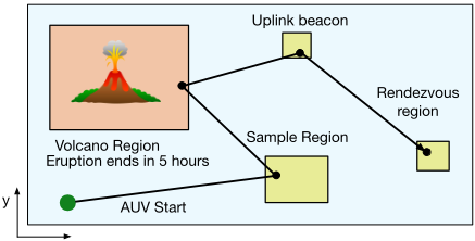
Figure 1: Example AUV mission.
tube representation of continuous effects from Kongming with the efficient solving method based on heuristic forward search and linear programs for consistency checking that COLIN uses. Scotty leverages the temporal flexibility of temporal planners and the control trajectory flexibility from model predictive control techniques to generate plans that are suited for robust execution.
1.1 Motivating Example
To motivate the need for a mixed discrete-continuous planner for robotic missions, we introduce an example scenario involving a scientific autonomous underwater vehicle (AUV) mission (Figure 1). In this mission the AUV has a deadline to complete two objectives before ascending to the rendezvous point. The AUV needs to take a sample in an specified region of interest and collect data of an ongoing underwater eruption site before the eruption ends, in five hours. The collected data needs to be uplinked to an optical underwater beacon, so that nearby scientists can analyze it as soon as possible.
This mission requires activities with discrete effects, such as collect-data, but also activities with continuous effects, such as navigate. In effect, in this mission we define the continuous state variables x and y that specify the position of the AUV at all times. Activities such as collect-data require the AUV to be in a specified region (constraints on x and y). The AUV can change its position using the continuous navigate activity. This activity varies the x and y state variables with time according to the control variable velX and velY, which are bounded and can be modified continuously. The hybrid planner needs to be able to reason with these continuous effects in order to take the AUV to the regions in which samples or data can be collected, and do it within their respective time windows. Table 1 shows an example fixed solution plan for this mission. In a later section, we discuss how to generate a flexible plan suitable for robust execution from the fixed solution plan for this problem.
In the next sections we describe Scotty's problem statement, its solution and how that solution is found.
2 Problem Statement
The input to the problem consists of the domain, initial conditions and goal. These extend PDDL 2.1 [Fox and Long, 2011] with some modifications that allow us to define activities with continuous effects that depend on bounded control variables. Similarly to PDDL 2.1, durative activities have a bounded controllable duration, discrete effects and continuous and discrete conditions defined at start, over all and at end. Continuous conditions are defined by linear inequalities over the state variables according to:
| t | Event | State | Control Variables |
|---|---|---|---|
| 0.0000 0.0001 0.0002 100.0002 100.0003 105.0003 105.0004 211.2504 289.9999 299.9999 300.0000 300.0001 337.5001 337.5002 342.5002 342.5003 430.0003 430.0004 440.0004 440.0005 | START-VOLCANO-ERUPTION START-DO-MISSION START-NAVIGATE-AUV END-NAVIGATE-AUV START-TAKE-SAMPLE END-TAKE-SAMPLE START-NAVIGATE-AUV END-NAVIGATE-AUV START-COLLECT-VOLCANO-DATA END-COLLECT-VOLCANO-DATA END-VOLCANO-ERUPTION START-NAVIGATE-AUV END-NAVIGATE-AUV START-UPLINK-VOLCANO-DATA END-UPLINK-VOLCANO-DATA START-NAVIGATE-AUV END-NAVIGATE-AUV START-ASCEND END-ASCEND END-DO-MISSION | x=0.0, y=0.0 x=0.0, y=0.0 x=0.0, y=0.0 x=400.0, y=75.0 x=400.0, y=75.0 x=400.0, y=75.0 x=400.0, y=75.0 x=150.0, y=500.0 x=150.0, y=500.0 x=150.0, y=500.0 x=150.0, y=500.0 x=150.0, y=500.0 x=300.0, y=545.0 x=300.0, y=545.0 x=300.0, y=545.0 x=300.0, y=545.0 x=650.0, y=420.0 x=650.0, y=420.0 x=650.0, y=420.0 x=650.0, y=420.0 | velX=4, velY=0.75 velX=-2.35, velY=4 velX=4, velY=1.2 velX=4, velY=-1.43 |
, where x′ = (x1, . . . , xnx , 1)T and c ∈ Rnx+1 is a vector of coefficients, with nx being the number of state variables of the system.
Our problem statement differs from PDDL 2.1 in the effects on continuous variables. Each activity has a set of control variables, which can be seen as continuous parameters - each of those constrained by lower and upper bounds. The continuous effects of the activity are similar to those of PDDL 2.1, except they are affected by the value chosen for the control variables. We restrict each continuous effect to involve only a single control variable, cvar, and thus each continuous effect can be defined by 〈x, cvar, k〉, where x is a state variable, cvar is a control variable, and k is a constant.
In the simple case, where a single continuous effect 〈x, cvar, k〉 is active from time tstart to time tend with cvar fixed to a constant value of c throughout the duration, then x(t), the value of state variable x at time t is defined by x(t) = x(tstart) + k · c · (t - tstart) with tstart ≤ t ≤ tend. Multiple continuous effects on the same state variable are
additive, and thus x(t) is defined by:
where Cx(t) is the sum of the values of control variables in active continuous effects modifying x at time t (represented by the set E).
where cvar(t) denotes the value chosen for the control variable cvar at time t. The navigate activity of the example AUV mission is shown in Figure 2. Note the bounded control variables velX and velY.
The problem initial conditions are given by the set of true propositions (P0) and an assignment to the state variables at the start (xi(0)). Finally, the goal consists of the discrete and continuous conditions that need to hold at the end.
(:durative-action navigate :control-variables ((velX) (velY)) :duration (and (<= ?duration 5000)) :condition (and (over all (>= (velX) -4)) (over all (<= (velX) 4)) (over all (>= (velY) -4)) (over all (<= (velY) 4)) (over all (<= (x) 700)) (over all (>= (x) 0)) (over all (<= (y) 700)) (over all (>= (y) 0)) (at start (AUV-ready))) :effect (and (at start (not (AUV-ready))) (at end (AUV-ready)) (increase (x) (* 1.0 (velX) #t)) (increase (y) (* 1.0 (velY) #t))))A fixed solution plan to the planning problem consists of a list of scheduled activities defined by the following properties: activity a, execution start time ta, duration da, and a trajectory of the value of each control variable of a from ta to ta + da, that is a function giving the value of each control variable at any given moment, caj(t) with ta ≤ t ≤ ta + da. Note that a fixed plan gives us the values of all the state variables (discrete and continuous) at every time t between 0 and the end of the plan - the state trajectory. We further require that all activity conditions are satisfied by the state trajectory at the appropriate times, as in PDDL 2.1.
A fixed plan is not robust: any small deviation during execution will cause the plan to fail. However, it is possible to use flexible plans that allow an executive to respond to small disturbances during execution. One such representation is Qualitative State Plans (QSP) [L´eaut´e and Williams, 2005]. A QSP is defined by a set of events (starts and ends of activities), along with simple temporal constraints and state constraints. Simple temporal constraints [Dechter et al., 1991] are of the form lb ≤ tj -ti ≤ ub, where ti and tj are execution times of events and lb, ub are a fixed lower and upper bound on the duration between ti and tj . State constraints specify legal values for continuous state variables at the start and end events of the state constraint, as well as the legal trajectories of continuous state variables and control variables. These trajectories specify the legal values of these at any moment in time between the events. Typically in robotic applications, these are given by the dynamics of the robot. For Scotty, these are limited to the linear form ∆x = cvar · ∆t with cl ≤ cvar ≤ cu.
Executives exist that can control a robot given a QSP as an input [L´eaut´e and Williams, 2005; Ono and Williams, 2008; Hofmann and Williams, 2006; 2015]. These executives choose the control variables and the execution times of events online, while ensuring that all constraints are met. Therefore, we focus on generating a flexible plan and leave its dynamic execution to the executive. In the next section, we review key ideas from existing planners that Scotty borrows.
3 Previous Work
In this section we briefly describe the approaches that Kongming and COLIN use to solve their planning problems. Scotty combines the best of these approaches to solve the hybrid planning problem with continuous control variables.
3.1 Kongming
Kongming solves the same planning problem as Scotty: actions are hybrid and their continous effects are modified by bounded continuous control variables. One of the main innovations introduced by Kongming consists in representing continuous effects with flow tubes, that are abstractions of the infinite number of trajectories that a continuous action can produce.
Another key innovation introduced by Kongming consists in the introduction of the Hybrid Flow Graph, the continuous analog to Graphplan's Planning Graph [Blum and Furst, 1997]. Hybrid actions connect initial state regions to goal regions after some fixed duration using the flow tubes generated from the system dynamics. Kongming expands the Hybrid Planning Graph with alternating action and fact layers until the goal conditions are non-mutex in the last fact layer. Kongming then encodes the problem as a mixed logic linear (non-linear) program that contains the system dynamics constraints on the state variables and logic constraints on binary variables for the discrete conditions and effects (similar to Blackbox's SAT encoding [Kautz and Selman, 1999]). Kongming alternates between trying to solve the ML(N)LP and adding additional layers to the graph until the ML(N)LP solver returns a solution.
Although Kongming's approach is innovative, it suffers from performance degradation issues in medium to large problems due to time discretization, as graph layers are discretized using a fixed time step. In problems in which the time horizon is moderately large, this involves creating many layers. As the number of layers increases, identifying mutex relations becomes exponentially more complicated. This also slows down significantly the ML(N)LP solver, as each additional layer adds many more additional variables and constraints. Later in this paper, we illustrate how this can become a problem very fast.
3.2 COLIN
COLIN solves temporal planning problems with continuous effects as defined in PDDL 2.1. Hybrid actions can have continuous time-varying effects, whose rate of change is specified by a fixed gradient.
In order to solve the planning problem, COLIN uses heuristic forward search. Every search state is tested for consistency with a Linear Program in which the real valued variables are the continuous state variables and the times at which actions are executed. The continuous linear time-varying effects and the temporal relations between actions are encoded as constraints. The linear program is also used at each step of the search to determine the minimum and maximum possible bounds for each state variable in order to prune actions that cannot possibly be feasible at that point of the search.
COLIN's heuristic is based on the Temporal Relaxed Planning Graph and delete relaxations. COLIN defines FF's analogous delete relaxation for continuous time-varying effects by only allowing state variable bounds to grow as a result of those continuous effects (bounds never get smaller). The heuristic value is the number of actions in the relaxed plan.
COLIN only supports continuous effects with fixed rates of change, according to the following equation:
x(tend) = x(tstart) + rate-of-change · (tend - tstart) (4)COLIN's formulation cannot handle bounded continuous rates of change (control variables). We can simulate this behavior by creating many equivalent continuous actions with discretized fixed rates of change. However, this solution is problematic as we will show later.
From COLIN we borrow the efficient solving approach based on linear programs for testing plan consistency and heuristic forward search. We also use a modified version of COLIN's heuristic. The key innovation of our approach consists in combining Kongming's more flexible representation of continuous actions based on flow tubes, with COLIN's more efficient solving approach based on heuristic forward search and no time discretization.
4 Approach
In order to find flexible solution plans, Scotty first finds a fixed plan. In this section we describe how Scotty uses flow tubes to represent continuous effects modified by continuous control variables, how fixed plans are found and, finally, how flexible plans are extracted.
4.1 Flow tube representation of continuous effects
As Kongming, our planner uses flow tubes to represent continuous effects modified by continuous control variables. Each activity can have multiple continuous effects, and each is represented by a flow tube. For Scotty, we limit flow tubes to operate on only one state variable. Flow tubes represent the reachable state space region, that is, the values that the state variable can take after the activity is started. We restrict continuous effects to linear time varying effects.
A flow tube f (dl, du, cvar, x, k) is defined by the following properties:
- minimum and maximum duration (dl, du), which are the minimum and maximum durations of the activity the flow tube belongs to.
- state variable x that the flow tube modifies.
- control variable cvar, is the activity control variable the flow tube is associated with. Recall that control variables are bounded (cl ≤ cvar ≤ cu).
- the scalar constant factor k that regulates the impact of the control variable on the state variable
If no other flow tubes affect state variable x between tstart and tend, then the reachable region of x represented by the flow tube f (dl, du, cvar , x, k) of an activity executed between tstart and tend is defined by the following equations:
where x(tstart) is the value of the state variable before the activity is executed. Note that, if the value of the control variable is constant during the execution of the activity, equation 5 reduces to x(tend) = x(tstart)+k·cvar ·(tend-tstart).
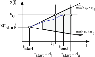
Figure 3 shows a flow tube. Note that any point in the shaded region (reachable region) can be reached at the end of the activity by carefully choosing the appropriate activity duration and control variable value. In the figure, we can see how the state value xe can be reached as fast as in tend = t1 if the control variable cvar is constant and takes its maximum possible value (cu), or as late as tend = tstart +du if cvar(t) takes smaller values.
Note that two or more flow tubes operating on the same state variable and belonging to the same or different ongoing activities can be active at the same time, having their effects combined. In general, if F represents the set of flow tubes belonging to ongoing activities in t ∈ [ta, tb], the following state evolution constraint between ta and tb holds:
where F is the set of flow tubes belonging to ongoing activities in t ∈ [ta, tb].
An important characteristic of flow tubes, is that they provide a compact encoding of all feasible trajectories. This property is exploited to find a fixed plan, as explained in the next section.
4.2 Finding a fixed solution plan
Now that we have defined how flow tubes represent continuous effects, we proceed to describe how fixed plans are found. In order to do that, Scotty uses a method based on heuristic forward search and linear programs for consistency checking, that is borrowed from COLIN. The main difference is that Scotty's continuous effects support control variables and are represented by flow tubes and, therefore, the state evolution constraints are different, as will be explained later.
Activities are represented by their start and end events, analogous to the start and end snap actions used by many temporal planners [Long and Fox, 2003; Coles et al., 2008]. In order to find a fixed plan, Scotty needs to find the ordered sequence of start and end events that takes the system from the initial conditions to the goal and the execution time of each event. Scotty also needs to find a trajectory for the values of each activity control variable between the start and end events of the activity (cvar(t) with tstart ≤ t ≤ tend).
Scotty finds trajectories for the control variables of an activity that are piecewise constant. The number of segments of these trajectories are given by 1+nev, where nev is the number of events that occur between the start and end events of the activity. Recall that, in general, the value of a control variable can vary within its bounds throughout the execution of the activity. However, Scotty only needs to find one solution at this step because, if the planning problem has a solution, there exists a solution with a piecewise constant control trajectory. The reason is that the state variables of the system only change due to the continuous effects of executing activities and are only constrained by the start, end and overall conditions of activities. Therefore, the constraints that state variables are subject to only change at events (starts or ends of activities). Moreover, these constraints are linear (inequalities as in (1)) and, therefore, the set of valid state variable assignments is convex. Because of that, if the problem can be solved, a fixed plan containing piecewise constant trajectories for the control variables is always a solution. We will show that a linear program formulation exists that can find such solutions.
As COLIN, Scotty uses heuristic forward search to find the sequence of start and end events that form a fixed plan, and linear programs to check the consistency of partial plans. The search uses Enforced Hill Climbing, which has proven to be effective in this type of problems [Hoffmann and Nebel, 2001]. However, because EHC is not complete, if no solution is found, Scotty can optionally try again with a complete algorithm such as best-first search.
Search states contain the set of propositions that are known to be true due to discrete effects, and are augmented with the ongoing activities list and the bounds for all state variables. The ongoing activities list keeps track of the activities that have started but not finished at that state and is needed to keep track of the active overall discrete and continuous constraints. The lower and upper bounds for the state variables are used to prune sections of the search tree that are necessarily not feasible. For example, if the start event of a certain activity a requires state variable x to be greater than 7 but the lower and upper bounds of x are 3 and 5 respectively, the search algorithm will not try to apply this event. However, an event having a x ≥ 4 condition will be tried in the search. Note that these state variable bounds are calculated for each state variable independently of the others. As a consequence, the fact that a constraint is satisfied by these bounds does not mean that the partial plan is necessarily feasible. Whether the partial plan is really feasible is only discovered when the linear program, used to test consistency, is solved.
Each search state defines a partial plan as the current sequence of start and end events, and is tested for consistency with a linear program. The partial plan is feasible if the linear program has a solution. In this linear program the decision variables are the event execution times and the values of the state variables at each event. The constraints include activity duration, start, end and overall conditions and state evolution constraints that are built from the current sequence of events. Table 2 shows the temporal and state constraints between Temporal Constraints
Total order of events:
For any pair of consecutive events i and j
Activity duration:
For every activity whose start and end events are i and j
where dl and du are the lower and upper bounds of the activity duration.
Activity conditions:
For every start or end event i
where ck ∈ Rnx+1 , x′i = (x1i , . . . , xnxi , 1)T and Ci is the set of active continuous conditions at event i: the start (or end) conditions of the activity, and the overall conditions of activities that started before i but whose end event occurs after i.
Table 2: Temporal and state constraints used in the consistency linear program. tk is the execution time of event k and xlk , the value of state variable xl at event k.
events. These constraints are the same ones that COLIN uses [Coles et al., 2012]. Scotty needs a different state evolution constraint, however, due to the presence of control variables. This constraint is given by the flow tube reachability equation (5). Because the values of the control variables can change during the activity execution, and the start and end times of the activity are variables of the linear program, this equation is not linear if control variables are decision variables of the linear program. However, we can redefine the reachability region of the flow tube with the following linear inequalities:
, where cl and cu are the bounds of the control variable. Note that min(k · cl, k · cu) represents the minimum rate of change of k · cvar and reduces to k · cl when k > 0. The more complicated expression is needed to preserve generality when k < 0. The same applies to the maximum rate of change. These linear inequalities represent the same flow tube reachability region described by equation (5) if each of the activity's control variables appear in only one continuous effect.
However, note that this is not always the case. Imagine an activity drive with its control variable speed. Assume drive has two continuous effects that are modified by the control variable speed. On one hand the state variable x is modified by the flow tube ∆x = speed ·∆t. On the other, the car's battery is drained according to ∆battery = -3 · speed · ∆t. Because the control variable speed that affects the battery drain is the same as the one that controls the rate of change in x, inequalities (13) and (14) can no longer represent the real state evolution of the system. These inequalities would artificially allow us to select at the same time a small value for the speed that drains the battery and a large one for the speed that makes the vehicle move fast. In these cases the reachability region needs to be represented with the original flow tube equations and the value of the control variable made a decision variable. Then the constraints become quadratic and the program is no longer linear. In its current implementation, Scotty only accepts activities in which this does not happen to keep the program linear but in the future, an appropriate solver will be used to handle quadratic constraints.
According to the previous discussion, Scotty uses the following state evolution constraints for state variable x between consecutive events i and j that consider that more than one continuous effect can be operating on x simultaneously:
where xk denotes the value of the state variable x at event k, tk is the execution time of event k and Axi→j is the set of continuous effects affecting x between events i and j. Recall that cl and cu denote the lower and upper bounds of each state variable.
Note that the values of the control variables are not decision variables of the linear program. However, for each pair of consecutive events 〈i, j〉, we can compute
, where C x i→j = ∑〈x,cvar,k〉∈Axi→j k · cvar. We can use this value to find piecewise constant assignments for each control variable between events i and j. Note that there could be infinitely many valid piecewise assignments if more than one continuous effect is affecting x. This is not a problem as Scotty only needs to find one at this step.
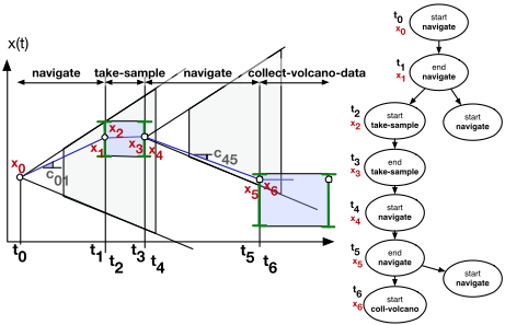
Figure 4 shows how flow tubes are handled in the linear program. The figure shows the values of state variable x as solved by the linear program at different search states. Activities' flow tubes and continuous conditions are shown. The consistency program is solved for each state in the search tree to determine the feasibility of the partial plan, and to extract the event times (t1 . . . t6), state variable values (x1 . . . x6), and control variables. These values keep changing as more steps are added to the plan during search. In order to find the state variable lower and upper bounds, the LP is solved twice per state variable (to minimize and maximize its value).
If the current search state is determined to be consistent, its heuristic value is computed and the state is added to the queue. If the state satisfies the goal conditions, a valid fixed plan has been found and Scotty proceeds to extract the flexible plan next. The last linear program used to extract the fixed plan tries to minimize the makespan of the plan, although a different optimization objective could be chosen.
The heuristic function used by Scotty is essentially the same used by COLIN, with minor modifications due to the use of control variables. The heuristic value for a state is the number of start or end events to reach the goal in the relaxed plan. The planning graph that COLIN expands keeps track of the state variables lower and upper bounds for each fact layer, with the caveat that activities can only grow these bounds, in a similar fashion to Metric-FF [Hoffmann, 2003]. COLIN calculates the positive gradient affecting each state variable by adding the positive rates of change of each ongoing activity (similarly with the negative gradient). In Scotty's case, these positive and negative gradients are found by adding the maximum (and minimum) rates of change given by the bounds of the control variables affecting each activity.
4.3 Extracting a QSP
The fixed solution plan obtained in the previous section is not robust: any deviation during execution may result in an infeasible plan. In this section we discuss how we extract a more flexible plan from the fully specified solution which can take advantage of the temporal and control flexibility of the problem.
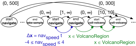
As described in the Problem Statement, we use Qualitative State Plans (QSPs) to describe such flexible plans. A partial QSP extracted from the solution plan of the example problem is shown in Figure 5. This QSP is a temporal network of events (starts and ends of activities). These events no longer have associated precise execution times as in the fixed plan, but are connected by temporal constraints that come from the duration constraints of the activities and the problem temporal constraints (such as collecting the volcano data before the eruption finishes in 300 minutes). Start and end events of activities with continuous effects (such as navigate) are connected by state evolution constraints that express restrictions on how variables can vary while the activity is being executed and what the bounds of the control variables are. Finally, events can have state constraints (conditions at start or end of activities), such as being in the rendezvous region at the end of the mission, and events can be connected by state constraints, that specify the feasible trajectories for the state variables between events (for example, being in the volcano region while the data is collected).
The QSP can be extracted by traversing the fixed plan schedule and annotating the temporal constraints (activity durations), state constraints (activity conditions) and state evolution constraints (continuous effects). This requires maintaining the total order of the events so that the discrete conditions of activities hold. Lifting a partial order plan from the grounded solution or, even better, using POPF's [Coles et al., 2010] approach of planning with partial order states is possible, and is considered for future work. In that case we would also have to annotate the discrete conditions as additional constraints in the resulting QSP.
Although we could extract a flexible plan like the one defined above from the solution of any temporal planner, the fact that Scotty operates with continuous control variables makes this plan much more useful. The advantage of Scotty compared to other temporal generative planners is that Scotty can reason with continuous control variables, making this flexible plans much more useful. In effect, this gives the executive the flexibility to choose not only the execution times of the events, but also the values of the control variables that modify the continuous effects. For example, if during execution it takes the AUV longer to take the sample than initially expected, the executive will be able to increase the navigation speed of the vehicle in order to ensure that the eruption data is collected before the event ends. In short, this provides the executive with two degrees of freedom to react to disturbances: the execution times and the control variables, as long as all state transition, activity conditions and time constraints are satisfied. Algorithms exist that can execute QSPs [Hofmann and Williams, 2015; 2006]. These algorithms execute the plan activities online by choosing the execution times of the events and the control variables, while making sure that all constraints are propagated forward and satisfied at all times.
5 Empirical Evaluation
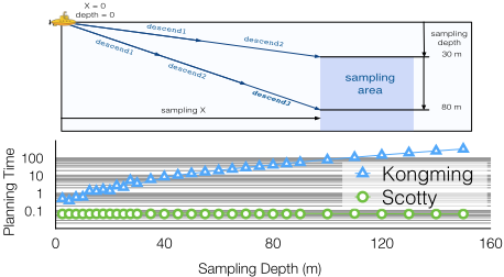
Scotty and Kongming can both reason with continuous effects modified by bounded control variables. In a previous section, we argued that Kongming's time discretization can hurt performance as the complexity of the problem increases. In Figure 6 we present a simple AUV sampling mission scenario that highlights this issue. The AUV needs to reach a certain depth range in order to take a sample. We parametrize this scenario in terms of the sampling depth. The AUV can use the action descend to modify its depth according to the bounded control variable descent-rate. Because Kongming discretizes time in constant time steps, increasing the target sampling depth forces Kongming to create additional fact
0
3.2. Preliminary Results
performance due to it's use of discrete time Example scenario:
Kongming
Higher depth (larger
distance) requires mo
time steps (layers) to
solution.
40
80
120
160
| 2D AUV 1 | 2D AUV 2 | 3DAUV | Firefighting 1 | Firefighting 2 | |
|---|---|---|---|---|---|
| Kongming | 3.633 | 9.736 | 13.063 | 1.505 | 20.202 |
| Scotty | 0.054 | 0.025 | 0.192 | 0.03 | 0.372 |
Table 3: Comparison between Kongming and Scotty in several domains. Results show planning time in seconds.
and action layers and, additionally, more variables that the ML(N)LP solver needs to consider. As a result, the performance of Kongming degrades very fast with the target sampling depth as shown in Figure 6. While Kongming's performance degrades very fast with depth, Scotty's performance is constant (and orders of magnitude better than Kongming's). This is expected, as Scotty does not discretize time and, therefore, is solving the same problem regardless of the depth. Table 3 shows Scotty's large performance advantage in other domains. These domains typically showcase one or more mobile robots moving in a 2D or 3D environment and completing objectives that involve visiting different locations.
On the other hand COLIN/POPF are efficient heuristic forward search planners that do not present the time discretization problem. However, they do not support continuous control variables, but fixed rates of change for continuous linear time evolving effects. Let us consider an example that shows why this is not desirable for robotic applications. Imagine that the AUV in the example mission needs to reach the volcano region (xmin ≤ x ≤ xmax) some prudent time after the eruption has ended so that it is safe to be nearby but before too long has passed, so that the collected data is still relevant (tmin ≤ t ≤ tmax). Let us consider that the robot can move with some speed (control variable) cl ≤ c ≤ cu. Note that in order to satisfy the constraints, the robot needs to move with some speed satisfying c∗l = xmin/tmax ≤ c ≤ c∗u = xmax/tmin. Because COLIN does not support continuous control variables, it would have to discretize the interval [cl, cu] into a set of discrete fixed rates of change. The problem would only be feasible if one of the discretized values fell inside the valid bounds [c∗min, c∗max]. Each discretized rate of change requires a new action, making the problem harder to solve. The required number of discretized rates of change can become arbitrarily large as different time and state constraints can modify the valid speed interval arbitrarily. Because Scotty supports continuous control variables, no discretization is needed and only one activity is sufficient as long as the interval given by the control variable bounds and the interval that contains the problem valid speeds have a nonempty intersection.
6 Conclusion
We have presented Scotty, a mixed discrete-continuous generative planner that fills the gap between high fidelity model predictive control approaches, that suffer from scalability problems, and temporal planners, that present an impressive performance on large problems at the cost of limited expressivity. Scotty uses flow tubes to compactly encapsulate continuous effects with continuous control variables, as Kongming, and heuristic forward search and a continuous time formulation, as COLIN. By avoiding discretization of either time or control variables, Scotty can reason with more expressive problems than COLIN and perform at least two orders of magnitude better than Kongming. Finally, Scotty produces flexible plans that are suitable for robust execution, as executives can exploit both temporal and control flexibility due to the presence of continuous control variables.
7 Acknowledgments
The work was partially supported by the Boeing Company under grant number MIT-BA-GTA-1. Enrique Fern´andez was also partially supported by "la Caixa Fellowship". The authors would also like to thank Andrew Coles for providing a PDDL grounder tool that was used for testing our planner.
@inproceedings{ijcai2015p224,
  title     = {Mixed Discrete-Continuous Heuristic Generative Planning Based on Flow Tubes},
  author    = {Fernández-González, Enrique and Karpas, Erez and Williams, Brian C.},
  booktitle = {Proceedings of the Twenty-Fourth International Joint Conference on
               Artificial Intelligence, {IJCAI-15}},
  publisher = {International Joint Conferences on Artificial Intelligence},
  editor    = {Qiang Yang and Michael Wooldridge},
  pages     = {1565--1571},
  year      = {2015},
  month     = {7},
  note      = {Main Track},
  url       = {https://ijcai.org/proceedings/2015/224},
}
TY - CPAPER TI - Mixed Discrete-Continuous Heuristic Generative Planning Based on Flow Tubes AU - Fernández-González, Enrique AU - Karpas, Erez AU - Williams, Brian C. T2 - Proceedings of the Twenty-Fourth International Joint Conference on Artificial Intelligence, IJCAI-15 PB - International Joint Conferences on Artificial Intelligence PY - 2015 SP - 1565 EP - 1571 UR - https://ijcai.org/proceedings/2015/224 ER -Copied
Machine-readable versions of this paper, for tools and AI agents:





