Path Integral Control by Reproducing Kernel Hilbert Space Embedding

1 Introduction

While solving general non-linear stochastic optimal control (SOC) and Reinforcement Learning (RL) problems remains challenging, some recent work by [Kappen, 2005] has identified a class of problems that admit closed form solutions. Although these solutions require evaluation of a path integral - equivalent to evaluation of a partition function, which in itself is a hard problem - they allow for the application of Monte Carlo and Variational methods, leading to several practical applications [Theodorou et al., 2010; Broek et al., 2011]. In the special case of linear dynamics and quadratic costs, the required path integral can be evaluated analytically based on linear operators acting on state vectors. Here, we show that, analogously, a suitable embedding of the path integral into a reproducing kernel Hilbert space (RKHS) allows its evaluation in terms of covariance operators acting on elements of the Hilbert space. While this in itself does not yield a tractable solution to the SOC problem, consistent estimators of the required operators give rise to efficient nonparametric algorithms.

The change of perspective from the direct estimation of the path integral (which previous applications of Monte Carlo methods aimed at) to estimation of operators allows to overcome several shortcomings of previous methods while maintaining many of their advantages. Most importantly, it can significantly reduce the sample complexity by splitting the problem appropriately into an invariant and task varying component, allowing efficient sample re-use across tasks and leading to a form of transfer learning - contrast this to the situation where any change in the task including, for e.g., different start states, necessitate acquiring new samples [Theodorou et al., 2010; 2009]. Additionally, the approach remains model-free, allowing its application to the RL setting. This is in contrast to variational [Mensink et al., 2010] or function approximation [Zhong and Todorov, 2011a; 2011b] approaches, from which it is further distinguished through convergence guarantees. The RKHS embedding make the operators state-dimensionality independent, leading to better scalability, while prior knowledge about both tasks and dynamics can be effectively incorporated by informing choices of sampling procedures and kernel.

It is worth noting that, while we choose to frame our approach in the context of path integral stochastic optimal control, it is not restricted to problems which fall into this class. The formalisms of linearly solvable MDPs by [Todorov, 2007], inference control by [Toussaint, 2009] and free energy control of [Friston et al., 2010] all require solving an underlying problem of equivalent form, making the methods proposed directly applicable in these contexts. Furthermore [Rawlik et al., 2012a] discusses a formulation which generalizes path integral control to derive an optimal policy for general SOC problems. Finally, while we focus on finite horizon problems, path integral formulations for discounted and average cost infinite horizon problems have been proposed by [Todorov, 2009], as well as by [Broek et al., 2010] for risk sensitive control.

Before proceeding, let us briefly outline the structure of the paper and give an informal overview about the key concepts involved in our approach. In Section 2 we first briefly review the formulation of a SOC problem in the path integral control framework of [Kappen, 2005]. This formulation has two specific properties relevant for our approach. First, it yields a closed form solution for the optimal policy in terms of a state desirability function (c.f. (3-4)). Second, this function can be expressed as a conditional expectation of the product of an immediate cost and a future desirability (c.f. (7)). By identifying this expression with an inner product in a RKHS, we can compute the desirability function. We formalise this notion in Section 3.1, where we address the model-based case and derive the analytical form of the RKHS based evaluation

(c.f. (13)). In Section 3.2, we consider the model-free case and discuss that this operator can be estimated from transition samples, leading to implementation in form of a finite dimensional inner product. To summarise, we solve the SOC problem by, (i) collecting transition samples and estimating the embedding operator, (ii) representing the desirability function and immediate cost as elements of RKHSs, (iii) recursively evaluating the desirability function as a series of inner products based on the estimated operator - n.b. this process involves a series of matrix multiplications - and finally (iv) computing the optimal controls based on the obtained desirability function. In Section 4, we build on this basic methodology and discuss a series of alternative estimators with either reduced computational costs or which allow for more efficient use of the sample data. Finally, in Section 5, we validate the proposed methods in experiments.

2 Path Integral Control

In this section we briefly review the path integral approach to stochastic optimal control as proposed by [Kappen, 2005] (see also [Kappen, 2011; Theodorou et al., 2010]). Let x 2 Rdx be the system state and u 2 Rdu the control signals. Consider a continuous time stochastic system of the form

where d⇠ is a multivariate Wiener process with E ⇥d⇠ 2 ⇤ = Q(x↪ t)dt, and f, B and Q may be non-linear functions. In particular note that the system is linear in the controls and both noise and controls act in the same subspace. We seek the best Markov policy, i.e., u(t) = ⇡(x(t)↪ t), with respect to an objective of the form

where T is some given terminal time, C÷ and C are a terminal and running cost respectively. The expectation is taken w.r.t. X⇡ (·), the paths of (1) starting in x and following policy ⇡. The quadratic control cost, given by H 2 Rdu⇥du , is further constrained by requiring it to satisfy Q = λBH-1BT for some constant scalar λ > 0.

It can be shown that for problems of this form, the optimised objective can be expressed as [Kappen, 2011]

where is a state desirability function given by the path integral

with (·↪ T) = exp¶-C÷(·)◁λ♦. The expectation in (4) is taken w.r.t. uncontrolled path of the dynamics (1), i.e. those under the policy ⇡0 (·↪ ·) = 0, starting in xt.

As a consequence of linear control with quadratic control cost and (3), the optimal policy ⇡⇤ (x↪ t) can be expressed directly in terms of as

making obtaining the main computational challenge for problems in this class.

Assuming we are only interested in the optimal controls at certain time points, say ¶t1↪▷▷▷↪n♦ with tn = T, it is sufficient to compute the set i(x) = (x↪ ti) and (4) admits a representation in terms of the finite dimensional distribution X = (X0 (t0)↪ · · · ↪X0 (tn)). Specifically using the Markov property of X0 (t) and marginalising intermediate states we obtain the recursive expression

with the expectation taken w.r.t. uncontrolled paths from xti to xti+1 . Note that -λ logΦi can be seen as the (optimal) expected cost for the problem of going from xti to xti+1 over the time horizon [ti↪ ti+1] under dynamics and running costs corresponding to those of the overall problem given in (2). Hence, the problem naturally decomposes into, on the one hand, a set of short horizon problems - or indeed a nested hierarchy of such Φ - and on the other hand, a set of recursive evaluations backwards in time.

3 Embedding of the Path Integral

We now demonstrate that (7) can be expressed in terms of linear operators in RKHS. While the exposition is necessarily short, [Hofmann et al., 2008] provide a more through treatment of the theory of RKHS, while [Smola et al., 2007], [Song et al., 2009; 2011] and [Fukumizu et al., 2011] provide the basic concepts on which we build.

We first concentrate on the evaluation of a single step, i.e., i given i+1, and derive model-based analytical expressions for the evaluation of i in terms of certain operators in RKHS.

3.1 Model-based Analytical One Step Path Integral Embedding

We essentially show that, in the model-based case, we may write (7) as an inner product in a RKHS. We proceed by first expressing expectations in terms of inner products in a RKHS, adapting the basic expression to conditional expectations and finally considering conditional expectations of functions of both the conditional and conditioning variable.

In general, we denote by Hk the RKHS of functions Z ! R associated with the positive semi-definite kernel k(·↪ ·). Further, let P Z be the set of random variables on Z. Following [Smola et al., 2007], we define the embedding operator E k : P Z !Hk by

which constitutes a direct extension of the standard embedding of individual elements z 2 Z into Hk , given by E k [z] = k(z↪ ·) commonly encountered.

In the problem under consideration, the interest lies with the evaluation of i given in (7) and hence, in a suitable embedding of Xi+1♣xi which would allow the required expectation to be expressed as an inner product in some RKHS. Although (9) can be directly applied - since for fixed xi, Xi+1♣xi is a simple random variable - it is convenient to consider a general conditional random variable Z♣y as a map Y ! P Z , yielding random variables over Z given a value y 2 Y, and define a conditional embedding U lk : Hl ! Hk s.t.

Note that here E l [y] = l(·↪ y), i.e., the standard embedding operator of elements y 2 Y used in kernel methods, and hence we may express conditional expectations as

Existence and a specific form for such an operator U satisfying (10) have been shown by [Song et al., 2009] and we omit the details of its derivation.

Unlike h in (11), the argument of the expectation in (7), specifically of Φ, is not only a function of the random variable, i.e., Xi+1, but also of the conditioning xi, and we can not apply (11) directly. We proceed by introducing an auxiliary random variable ˜X such that P( ˜X↪Xi+1♣xi) = P(Xi+1♣xi)δ ˜X=xi with δ the delta distribution, hence for all h 2 Hk

Note that treating xi as constant leads to an alternative formulation. This, although equivalent in the analytical setting, does however not immediately yield a practical empirical estimator.

We may now turn to substitution of the specific argument encountered in (7) for the generic function h. Specifically, assume H ↪Hφ , s.t. 2 H , Φ 2 Hφ , are given 1 . To account for the mismatch in the arity of functions in these spaces, H may be trivially extended toH 0 , a space of functions Rdx ⇥Rdx !R, using the kernel 0 ((u↪ v)↪ (u0 ↪ v0 )) = (u↪ u0 ), i.e., we identify H and its tensor product with the RKHS of constant functions. Hence, taking the embedding of Xi+1↪ ˜X♣xi into Hw = Hφ ⌦H 0 in which the product function of Φi, i+1 resides, we rewrite (7), using (12) and

1 n.b., Hφ is a space of functions Rdx ⇥ Rdx ! R, while H contains functions Rdx ! R

where k is some kernel over Rdx of our choosing. As will become apparent in the following (see (16)), it is convenient for computational reasons to take k to be as it allows for reuse of pre-computed matrices over the recursive evaluation of estimates of .

Algorithm 1: Basic Backward Algorithm

3.2 Model-free Finite Sample Estimates

Evaluation of the embedding of random variables and in our case U - thus also of the path integral embedding (13) - requires evaluation of expectations of kernels and remains therefore, in most cases, intractable. Further it requires exact analytical knowledge of the system dynamics (1). However, as we shall see it is straightforward to form empirical estimates, leading to practical algorithms.

Specifically let D = ¶(x↪ x0 )1▷▷▷m♦ be a set of i.i.d. state transition samples of the uncontrolled dynamics (c.f. Section 2), e.g., a sample set obtained from trajectory executions under the policy ⇡0 . It can be shown [Song et al., 2009], that a regularized estimate of U kw is given by

where ✏ represents a regularization parameter and g X ,gw X 0 and G XX represent the vectors of embeddings and Gramian on the sample data D respectively, i.e., [g X ]i = φ(xi↪ ·) and [G XX ]ij = (xi↪ xj). In order to evaluate (13), we furthermore require the representations of Φi and i+1 in their respective RKHSs. As we evaluate recursively, we may assume the empirical estimate of i+1 to be already given as ¯ i+1 = Pxj2X [↵i+1]j (xj↪ ·) = g X ↵i where ↵i+1 is a vector of weights. Similarly we will assume the representation of Φi in Hφ to be given by gφB β for some weights β and set B. While such a representation is, under the assumption Φi 2 Hφ , guaranteed to exists we will see that it is not necessary to explicitly compute it. Substituting the empirical operator ˆ U kw of (14), together with the kernel expansions of Φi and i+1 into (13), matrix algebra yields the empirical estimate of i(x) as

with weights ↵i given by

where ⊙ denotes the Hadamard product. While (16) provides the means for recursive evaluation of the weights ↵, it remains to obtain corresponding representation of Φi given by β. However, we note the term involving the representation of Φi can be written as

This means obtaining an explicit representation of Φ in terms of the kernel expansion in Hφ is not necessary, rather it is sufficient to be able to evaluate Φi at the sample data D - equivalent to evaluating the cost function (cf. (8)).

Importantly, note that ¯ i is a finite weighted sum of kernels, hence, ¯ i 2 H , which directly allows a recursive computation of all ¯ 1▷▷▷n. Furthermore, all required matrices are functions of the sample data only and, as such, can be precomputed. The resulting algorithm for computation of the desirability function ¯ is summarised in Algorithm 1. Using (5), it is then straightforward to obtain an approximate optimal policy for fine discretisations of the problem.

4 Efficient Estimators

The basic estimator (16) has several drawbacks. For one it has a relatively high computational complexity of O(m3 ) for the matrix inversion, only required once if the same D is used in each time step, and subsequently O(m2 ) per iteration. Additionally, sample data under the uncontrolled dynamics is required, thus not allowing for off-policy learning. However, these problems can be addressed with alternative estimators for U based on low rank approximations [Song et al., 2011] or importance sampling [Rawlik et al., 2012b] We choose to ommit the discussion of these in order to address a, in our opinion, often overlooked aspect of efficiency when solving varying problems under the same dynamics. In practice, tasks are not performed in isolation, rather varying instances of often related problems have to be solved repeatedly, e.g., an optimized single reaching movement is of limited use since complex interactions require a series of such movements with changing start and target states. Previous approaches generally assume re-initialisation for each problem instance, e.g., Monte Carlo methods require novel samples, even under such trivial changes as the start state. In the following, we discuss extensions to the proposed method which improve sampling efficiency in exactly these cases, allowing efficient sample reuse over repeated applications.

4.1 Transfer Learning via Transition Sample Re-use

A limitation of the estimator arising in practice is the necessity of evaluating Φ at the training transitions (cf. (16) and (17)) which, in general, may be infeasible. It is therefore desirable to obtain an estimator based on evaluation of Φ on a separate, ideally arbitrary, data set D0 . Observe that

where Z is some free random variable with support on Rdx ⇥ Rdx and we used an empirical estimator based on a data set D0 = ¶(x↪ x0 )1▷▷▷m0♦ of i.i.d. samples from Z (often in practice D0 ✓ D). As indicated evaluation of the r.h.s. only requires evaluation of Φ at elements of D0 , hence substituting into (16) gives the desired result. In particular we are now able to pre-compute and re-use the inverse matrix of (16) across changing tasks and, assuming time stationary dynamics, across different time steps. This is of importance for efficient estimation in, e.g., the RL setting where incurred costs are known only at observed transitions or in cases where Φ can be freely evaluated but it is expensive to do so, while generating large sets of transition samples may be comparatively cheap, e.g., the case of simple kinematic control where cost evaluation requires collision detection. Note that this form makes explicit use of the kernel φ, and while we may not be able to guarantee Φ 2 Hφ , by choosing a kernel such that the projection of Φ onto Hφ is close to Φ, we can expect good results.

4.2 Task Augmented Sampling

We now turn to the question of the sampling distribution. While, in general, samples are required from the task agnostic dynamics X0 , a task often induces regularities which suggests more suitable sampling distributions. In particular, considering the role Φ takes in (16) (via (17)) as a weight vector, it appears desirable, akin to importance sampling, to concentrate samples in regions of high Φ. Obviously Φ can be used to guide the choice of the sampling distribution, however, in the context of repeated tasks we can go further and incorporate Φ partly into the sampling process allowing, amongst others, for incremental learning of the task.

Consider the specific situation where one wishes to execute several task instances of a generic skill. This situation is often characterised by an invariant cost component relating to the skill and a task specific cost component - if one looks at walking as an example, we wish to stay balanced in each step but the foot placement target will differ from step to step. Formally assume the state cost decomposes as

where ✓ parametrises the task. In this case, we may write the path integral (4) as

where the expectation is now taken w.r.t. path of X⌫ , which are the dynamics under the optimal policy under the invariant skill component of the cost. This allows for both, incremental learning and, using the results of Section 4.1 the transfer of samples between varying tasks sharing a skill component.

5 Experimental Validation

5.1 Double Slit

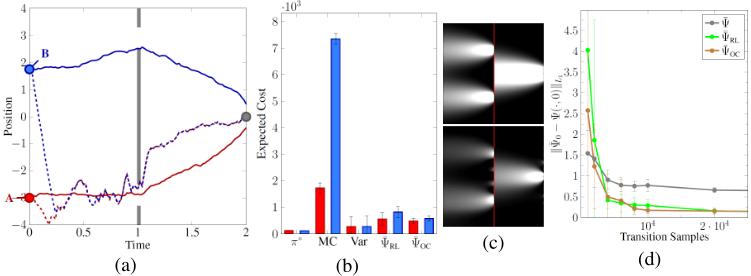
We first consider the double slit problem, previously studied by [Kappen, 2005] to demonstrate Monte Carlo approaches to path integral control. The problem is sufficiently simple to allow for a closed form solution for to be obtained, but complex enough to highlight the shortcomings of some previous approaches. The task concerns a particle moving with constant velocity in one coordinate, while noise and controls affects it's position in an orthogonal direction. The aim is to minimise the square error to a target position at some final time, while also avoiding obstacles at some intermediate time, as illustrated in Fig. 1(a). Specifically, the one dimensional dynamics are dx = u + d⇠ and the cost is given by

↪

where ! is a weight. We considered a discretisation with time step 0▷02s, i.e. 100 time steps.

We compare the true optimal policy to those obtained using two variants of the proposed estimator, ¯ OC and ¯ RL. The latter is based on a RL setting, learning from trajectory data without access to the cost, and uses the approach for sample sharing across time steps discussed in Section 4.1. Meanwhile, ¯ OC is based on single transitions from uniformly sampled start states and uses knowledge of the cost function to evaluate Φ in each step. In both cases we use the low rank approximation and square exponential kernels (x↪ y) = exp¶(x - y)2 ◁γ♦ with γ set to the median distance of the data. For comparison, we also consider two alternative approaches - firstly, the trajectory based Monte Carlo approach of [Theodorou et al., 2009], using the same number of trajectories as used in the RL setting and on the other hand, a variational approximation, specifically a Laplace approximation to the true to obtain a linear approximation of the optimal policy. As can be seen in Fig. 1(b), the proposed approach leads to policies which significantly improve upon those based on the alternative Monte Carlo approach and which are comparable to those obtained from the variational approximation, which however was computed based on knowledge of the true . In particular, note that the proposed approach makes better use of the sample provided, finding a policy which is applicable for varying starting positions, as illustrated in Fig. 1(a). As seen from the trajectories in Fig. 1(a), the Monte Carlo approach on the other hand fails to capture the multi modality of the optimal policy leading to severely impoverished results when applied to starting point B without sampling a new data set (c.f. Fig. 1(b)). The variational approximation on the other hand similarly requires recomputation for each new starting location, without which results would also be significantly affected.

To illustrate the dependence of the estimate on the sample size we compare in Fig. 1(c) the evolution of the L1 error of the estimates of at time t = 0. Sample size refers to total number of transition samples seen, hence for ¯ RL the number of trajectories was the sample size divided by 100. In order to also highlight the advantages of the sample re-use afforded by the approach in Fig. 4.1, we also compare with ¯ , the basic estimator given data of the same form as ¯ RL, i.e. recursive application of (16) without sample sharing across time steps.

5.2 Arm Subspace Reaching Task

We consider reaching tasks on a subspace of the end-effector space of a torque controlled 5dof arm, simulating constrained tasks such as, for e.g., drawing on a whiteboard or pushing objects around on a table. Here the skill component consists of moving with the end-effector staying close to a two dimensional task space, while the task instances are given by specific reach targets. The task space used is a linear subspace of the end effector space, n.b., hence, a non linear subspace of the joint space, and the cost comprises the two components

where '(·) is the mapping from joint to end-effector coordinates, J & j define the task subspace, ✓ specifies the reaching target and !'s are weights. We again consider position control over a 2s horizon with a 0.02s discretisation.

This task is challenging for sample based approaches as the low cost trajectories are restricted to a small subspace, necessitating large sample sizes to obtain good results for an individual reaching target, even if, as suggested by [Theodorou et al., 2009] and done here, an inverse dynamics policy is used which significantly improves end-effector exploration. However, concentrating on the case of changing targets, we exploit the ideas from Section 4.2 by assuming the operators have been estimated under the skill augmented dynamics 2 (cf. (19)), and consider subsequent learning for a novel task using the estimator from Section 4.1, utilising the already estimated operators in two ways. On the one hand, they are directly used in the calculation of ¯ , on the other hand, noting, that as the trajectories are only required to provide D0 , hence do not have to be sampled under a specific policy, we use the policy arising when considering Cskill only, i.e., the skill policy associated with ¯ computed using the given operators and Ctask(·) = 0.

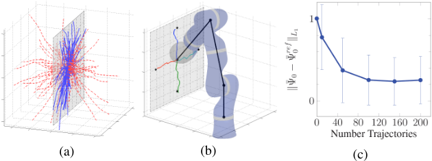
The advantage of sampling under the skill policy is illustrated in Fig. 2(a) where sample trajectories under both the skill and null policy are shown, demonstrating that the former more effectively explores the task relevant sub space. Mean trajectories for policies learned from 100 trajectories for a set of tasks are illustrated in Fig. 2(b). In Fig. 2(c) we plot the L1 error of ¯ as a function of trajectories averaged over ten ✓. As the true is not available for this task we show the error w.r.t. a ¯ ref 0 computed from 5000 trajectories, principally to illustrate the rapid convergence of the estimator.

6 Conclusion

We have presented a novel approach for solving stochastic optimal control problems which are of the path integral control form using Monte Carlo estimates of operators arising from a RKHS embedding of the problem, leading to a consistent estimate of . While direct application of Monte Carlo estimation to point evaluation of also yields a consistent estimate, it is impractical for computation of controls for anything but simple problems, requiring a trajectory sample for each state at which an action is to be computed. Although previous work, e.g. by [Theodorou et al., 2009;

2 n.b., while here such a sample is generated explicitly, the more time consuming approach of using the importance sample based estimator and collecting a sample under X0 could be used

2010], has suggested approaches to overcome the problem of sample complexity, these sacrifice consistency in the process and we demonstrate that the proposed approach significantly improves upon them in terms of generalization to a policy (cf. results in Fig. 1(a,b)). We furthermore show that the presented estimators allow for sample re-use in situations which previously required an entirely novel sample set. In particular we consider transfer in cases where execution of several, potentially related, tasks on the same plant is required, demonstrating that it is possible to exploit samples from all tasks to learn invariant aspects.

Note that as Φ itself defines a local optimal control problem, an alternative perspective on the proposed method is as a principled approach to combining solutions to local control problem to solve a more complex large scale problem. In future work we aim to elaborate on this interpretation by combining the methods presented with alternative approaches, e.g., variational methods, which may be sufficient to provide good estimates for the comparatively simpler local problems.

The choice of kernel has been largely ignored here, but one may expect improved results by making informed kernel choices based on prior knowledge about the structure of the problem.

In related work, [Gr¨unew¨alder et al., 2012] recently proposed to utilise RKHS embeddings of the transition probability for computation value functions in MDPs. While the methodologies are in principle comparable, our work goes beyond that of Gr¨unew¨alder et al. in several aspects. For one, we directly obtain the optimal controls, rather then just computing the value function, leaving obtaining optimal controls to be performed by explicit maximisation. Furthermore Gr¨unew¨alder et al. concentrate on finite state problems (where computation of the optimal u is simpler). We meanwhile, concentrate on the harder continuous problem and in particular, provide convergence guarantees in this setting. Finally, we make a contribution to the efficient estimation of the required quantities by exploiting the structure of the problem, allowing efficient sample re-use and transfer.