
Machine-Learning-Based Circuit Synthesis
Proceedings of the Twenty-Third International Joint Conference on Artificial Intelligence. Pages 1635-1640.
© 2013 International Joint Conferences on Artificial Intelligence
Abstract
Multi-level logic synthesis is a problem of immense practical significance, and is a key to developing circuits that optimize a number of parameters, such as depth, energy dissipation, reliability, etc. The problem can be defined as the task of taking a collection of components from which one wants to synthesize a circuit that optimizes a particular objective function. This problem is computationally hard, and there are very few automated approaches for its solution. To solve this problem we propose an algorithm, called Circuit-Decomposition Engine (CDE), that is based on learning decision trees, and uses a greedy approach for function learning. We empirically demonstrate that CDE, when given a library of different component types, can learn the function of Disjunctive Normal Form (DNF) Boolean representations and synthesize circuit structure using the input library. We compare the structure of the synthesized circuits with that of well-known circuits using a range of circuit similarity metrics.
- [Aguirre et al., 1999] Arturo Hernández Aguirre, Bill P. Buckles, and Carlos A. Coello. A genetic programming approach to logic function synthesis by means of multi- plexers. In Proceedings of the 1st NASA/DOD workshop on Evolvable Hardware, EH'99, pages 46-, Washington, DC, USA, 1999. IEEE Computer Society.
- [Aguirre et al., 2003] Arturo Hernández Aguirre, Edgar C. González Equihua, and Carlos A. Coello Coello. Syn- thesis of Boolean functions using information theory. In Proceedings of the 5th international conference on Evolv- able systems: from biology to hardware, ICES'03, pages 218-227, Berlin, Heidelberg, 2003. Springer-Verlag.
- [Bernasconi et al., 2012] Anna Bernasconi, Valentina Ciri- ani, Valentino Liberali, Gabriella Trucco, and Tiziano Villa. Synthesis of p-circuits for logic restructuring. In- tegration, the VLSI Journal, 45(3):282-293, 2012.
- [Brayton et al., 1984] Robert King Brayton, Alberto L. Sangiovanni-Vincentelli, Curtis T. McMullen, and Gary D. Hachtel. Logic Minimization Algorithms for VLSI Synthe- sis. Kluwer Academic Publishers, Norwell, MA, USA, 1984.
- [Curk et al., 2005] Tomaž Curk, Janez Demšar, Qikai Xu, Gregor Leban, Uros Petrovič, Ivan Bratko, Gad Shaulsky, and Blaž Zupan. Microarray data mining with visual pro- gramming. Bioinformatics, 21:396-398, February 2005.
- [Gan et al., 2008] Zhaohui Gan, Tao Shang, Gang Shi, and Chao Chen. Automatic synthesis of combinational logic circuit with gene expression-based clonal selection algo- rithm. In Proceedings of the 2008 Fourth International Conference on Natural Computation -Volume 06, pages 278-282, Washington, DC, USA, 2008. IEEE Computer Society.
- [Hansen et al., 1999] Mark Hansen, Hakan Yalcin, and John Hayes. Unveiling the ISCAS-85 benchmarks: A case study in reverse engineering. IEEE Design & Test, 16(3):72-80, 1999.
- [Hong and Muroga, 1991] Sung Je Hong and Saburo Muroga. Absolute minimization of completely specified switching functions. IEEE Trans. Comput., 40:53-65, January 1991.
- [Koza et al., 1996] J.R. Koza, D. Andre, F.H. Bennett III, and M.A. Keane. Use of automatically defined functions and architecture-altering operations in automated circuit synthesis with genetic programming. In Proceedings of the First Annual Conference on Genetic Programming, pages 132-140. MIT Press, 1996.
- [McCluskey, 1956] E. J. McCluskey. Minimization of Boolean functions. The Bell System Technical Journal, 35(5):1417-1444, 1956.
- [Parhami, 2009] Behrooz Parhami. Computer Arithmetic: Algorithms and Hardware Designs. Oxford University Press, Inc., New York, NY, USA, 2nd edition, 2009.
- [Roth, 1958] J.P. Roth. Algebraic topological methods for the synthesis of switching systems I. Trans. Amer. Math. Soc, 88(2):301-326, 1958.
- [Temes and Lapatra, 1977] G.C. Temes and J.W. Lapatra. In- troduction to Circuit Synthesis and Design, volume 15. McGraw-Hill, 1977.
- [Zupan et al., 1999] Blaž Zupan, Marko Bohanec, Ivan Bratko, and Janez Demšar. Learning by discovering con- cept hierarchies. Artif. Intell., 109:211-242, April 1999.
References were extracted automatically from the PDF and may contain errors.
Full text extracted automatically from the PDF; figures, tables and equations may differ. The PDF is the version of record.
1 Introduction
Logic (or Boolean Function) Synthesis is a well-known problem, and is a key to developing circuits that optimize a number of parameters, such as depth, energy dissipation, reliability, etc. The problem can be defined as the task of taking a collection of components from which one wants to synthesize a circuit that optimizes a particular objective function. This problem has been addressed since Roth [Roth, 1958]. More recent work has focused on synthesis of circuits jointly optimizing a complex objective function [Temes and Lapatra, 1977; Zupan et al., 1999], optimization via genetic algorithms [Koza et al., 1996; Aguirre et al., 2003], and on circuit re-engineering, e.g., [Bernasconi et al., 2012].
Circuit synthesis is related to, but strictly more general than, Boolean minimization, on which there has been significant work (e.g., using the Quine-McCluskey method [McCluskey, 1956]). Rather than being given a function to optimize, we must jointly create the function and optimize it; in addition, we may want to address many other tasks in the synthesis process; such tasks include (1) optimize properties beyond just the number of gates that Boolean minimization addresses (e.g., circuit area, depth), (2) add components not present in the given function, and (3) design nested hierarchical structures in the device.
We aim to automate the process of generating circuits from component libraries. We propose a machine learning approach. Prior work has used genetic algorithms, which do not converge well [Aguirre et al., 1999; 2003]. We adopt a decision tree approach, and in particular, an iterative greedy algorithm that adds the most efficient component in terms of model size. Our approach is not restricted by a pre-defined library of component types but uses a library that can dynamically grow, and thus keeps the model size small.
Our approach has several important applications: (1) In reverse engineering, engineers can shorten the process of revere-engineering. For instance, automating this process could significantly reduce the time duration of unveiling key systems; e.g., it could emulate the reverse engineering of the ISCAS-85 benchmarks [Hansen et al., 1999]. (2) In modelbased synthesis, automating the process of Boolean function synthesis is needed for model-based systems. The existence of a model is a basic requirement for model-based systems. Unfortunately, in many cases such a model does not exist. (3) In model-based diagnosis, this approach can take a system function and optimize its diagnostics properties, e.g., diagnosability, fault tolerance, failure probability, etc.
Our contributions are as follows. We propose a novel machine learning approach for Boolean function decomposition for the case of multi-level logic synthesis. We propose reverse engineering of Boolean formulas rather than addressing designing problems. We cope with multiple output functions rather than a single output. We implement a method that uses a library of different component types which can be dynamically increased with new types of components. Finally, our algorithm is empirically evaluated through various circuits.
2 RelatedWork
The task of composing a model from components to achieve a goal function is known in the electrical and computer engineering literature as logic synthesis. Logic synthesis is a process for converting a high-level specification of circuit behavior, typically register transfer level (RTL), into a design implementation, which can be represented in terms of logic gates.
In two-level logic synthesis the goal is to represent a Boolean function by at most two gate levels between a primary input and a primary output. This can be achieved by representing the function as a DNF (in terms of the engineering literature: sum of products). Known methods for this task are Quine-McCluskey [McCluskey, 1956] to compute the exact prime implicants of the goal formula and heuristic methods like ESPRESSO [Brayton et al., 1984] and MINI [Hong and Muroga, 1991] which compute near-minimal prime implicants. Amajor limitation of this approach is that two-level logic circuits are of limited importance in a most real-world applications, e.g., in very-large-scale integration (VLSI) design, since most designs require multiple levels of logic.
Another attempt to solve the multi-level logic synthesis is by genetic algorithms. Aguirre et al. [Aguirre et al., 1999; 2003] propose to use a multiplexer as the only design unit, defining any logic function. They first explore a feasible design and then minimize the circuit. Gan et al. [Gan et al., 2008] present the genetic-based algorithm denoted Gene Expression-based Clonal Selection Algorithm (GECSA), which combines the advantages of the Clonal Selection Algorithm (CSA) and Gene Expression Programming (GEP), overcoming some drawbacks of GEP. These works focus on a single output function, we on the other hand, show a machine learning approach which solves multiple logic functions in one circuit. In addition, a known drawback of genetic algorithm is the long time of convergence. Unfortunately, even the above papers demonstrate their approach only for a few simple circuits.
Zupan et al. [Zupan et al., 1999] present a new machine learning approach that infers a target function from a set of training examples. It is represented in terms of a hierarchy of intermediate, less-complex concepts and their definitions. The method is inspired by the Boolean function decomposition approach to the design of switching circuits by suboptimal heuristic algorithms. Since this algorithm is not restricted to a given set of gates, it actually tries to decompose the function to artificial sub-functions. We adopt the hierarchical approach but redesign it to solve the multi-level logic synthesis consistently by a given library of component types.
3 Concepts and Definitions
We start by presenting a set of definitions that are designed to facilitate the exposition of algorithms for automated reasoning.
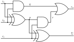
Figure 1 shows an implementation of a full-adder, represented by the function F(i1, i2, ci) = (q ⇔ i1 ∧ i2) ∧ (p ⇔ i1 ⊕ i2) ∧ (Σ ⇔ p ⊕ ci) ∧ (co ⇔ q ∨ (p ∧ ci)).
Definition 1 (Component) A component COMP, 〈F, IN, OUT〉, is specified using a Boolean function F over a set of variables Z, and input/output variables, IN, OUT ∈ Z.
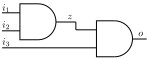
Boolean functions that model components are often represented graphically, by using the same symbols as in a standard computer arithmetic schoolbook [Parhami, 2009]. Figure 2 shows a component that implements a three-input AND gate by using two two-input ones. The Boolean function that is shown in Fig. 2 is F(i1, i2, i3) = (o ⇔ z ∧ i3) ∧ (z ⇔ i1 ∧ i2) where IN = {i1, i2, i3}, OUT = {o}, and z is an internal variable. We may omit specifying which variables are input and output, when that is clear from the context or from the common use (of an AND gate, for example).
Definition 2 (Component Library) A component library L is defined as a set of components.
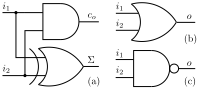
Figure 3 shows a component library consisting of a halfadder, a two-input OR gate and a two-input NAND gate. In our problem formulation, there are no restriction on the contents of the component library, i.e., it is a set of arbitrary multi-output Boolean functions. It is not necessary for a component library to contain a functionally complete subset of components (the two-input NAND gate in the component library shown in Fig. 3, for example, can be used to express any Boolean function, but that is not a requirement in our framework).
Definition 3 (SystemDescription) A system description SD, 〈L, G〉 is defined as a vertex-labeled and edgelabeled direct acyclic graph G = 〈V,E〉 such that V = {PI ∪ PO ∪ V ′} and if v ∈ V ′ , then v ∈ L.
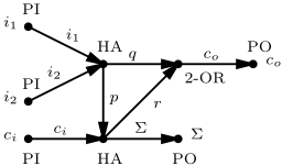
System description graphs contain a set of primary input vertices (PI), a set of primary output vertices (PO) and a vertex for each component. The graph edges are labeled with the names of the Boolean function variable names.
Figure 4 shows a system description of the full-adder circuit shown in Fig. 1, built from components drawn from the Fig. 3 library.
A system description SD is equivalent to exactly one Boolean function as shown in the following definition.
Definition 4 (Composition) Given a system description SD = 〈L,G〉, G = 〈V,E〉, a composition C(SD) of SD is a Boolean function (f1 ◦ · · · ◦ fn)(x1, . . . , xm) such that n = |V | - |PI| - |PO| and for each fi ∈ {f1, . . . , fn}, there is an isomorphic function f ′ i ∈ L. The primary inputs and primary outputs of f1, . . . , fn are the respective edge labels in G and the internal variables in f1, . . . , fn are unique.
In the above definition the variables {x1, . . . , xm} are all internal variables, i.e., {x1, . . . , xm} = V \ {PI ∪ PO}.
The composition of the system description in Fig. 4, for example, is a Boolean function that is composed of two halfadders, and a two-input OR gate. The i1 and i2 inputs of the half-adder in the component library shown in Fig. 3 are renamed to p and ci for one of the instances.
Definition 5 (SystemDecomposition) Given a component library L and a Boolean function S, a system decomposition S-1 of S is a system description SD = 〈L, G〉 such that S ≡ C(SD).
By equivalent function we mean that, since S and C(SD) have the same primary inputs and primary outputs, a valuation φ(S) = 1 iff φ(C(SD)) = 1. Note that the problem of computing if two Boolean functions are equivalent is computationally very hard.
Computing decompositions of a given Boolean function is the main problem discussed in this paper. Certain decomposition are preferable, i.e., these minimizing some optimality criterion such as number of elementary functions (number of internal nodes in the resulting system description), a cost function, etc. In this paper, the optimality criterion minimizes the number of nodes in G.
4 DecompositionMetrics
We are interested in using circuit decomposition for discovering "structure" in unknown Boolean functions. To evaluate the performance of our algorithms we introduce a class of basic similarity metrics. In this case we (1) use a specified system description SD to obtain a "flat" representation, e.g., a Disjunctive Normal Form (DNF), (2) decompose the "flat" representation, obtaining a new system description SD′ and (3) use SD and SD′ to compare the metrics described next. We denote the SD graph with G = 〈V, E〉 and the SD′ graph with G′ = 〈V ′ , E′ 〉.
We can use the graph degree distribution, where the degree of a node in a graph is the number of edges incident on that node. Since a circuit graph is directed, nodes have two different degrees, the in-degree, which is the number of incoming edges, and the out-degree, which is the number of outgoing edges. The degree distribution P(k) of a graph is the fraction of nodes in the graph with degree k (in this case we do not take into consideration the orientation of the edges). Thus if there are n nodes in total in a network and nk of them have degree k, we have P (k) = nk/n.
The mean degree of a graph is given by
where V is the set of all nodes and |v| is the degree of a node v.
The graphs that we deal with are attributed graphs, with the nodes having a component-type attribute, which we denote as λ(v) for v ∈ V . Given this, we can define a component-type distribution, which is
given component types 1, . . . , k for a fixed ordering of types. For example, for the full-adder circuit with gate-type ordering (AND, OR, XOR), we have the distribution (0.4, 0.2, 0.4).
We denote the SD graph with G = 〈V,E〉 and the SD′ graph with G = 〈V ′ ,E′ 〉. We compare a number of graphtopology ratios, which we define as follows:
- Node Ratio: ≡ V/V ′ .
- Component-type distribution ratio:
whenever Λi(v) is not zero.
- Degree distribution ratio, where well-defined, i.e., P(k) ̸= 0.
- Average Vertex Degree Ratio = ¯k ¯k′ .
We use all of the above metrics to measure the quality of a decomposition. In this paper we do not supply weights for the different metrics and we do not combine them. For example, if one introduces a component cost function, it should be taken into consideration when combining the componenttype distribution ratios of the different component types.
5 Circuit Decomposition
We first discuss some general properties of the Boolean function decomposition problem and then we give an efficient algorithm for computing decompositions.
5.1 Relation to Known Decompositions
One question that arises is the type of component library that is necessary for decomposition. It turns out that we can use a library L consisting of the well known functionally complete set of gates (Boolean operators), i.e., L can consist of the sets { AND, NOT }, {NAND}, or {NOR}.
Certain decompositions are preferable, i.e., these minimizing some optimality criterion such as number of elementary functions (number of internal nodes in the resulting system description), a cost function, etc. We can thus generalize our notion of system decomposition to include a preferred system decomposition, which is a system decomposition that is optimal with respect to an optimality criterion O.
Given these definitions, it is straightforward to reduce the problem of circuit synthesis to several well-known Boolean optimization problems. In particular:
- Consider a component library that consists of Boolean functions of the following kind:
for n = 1, 2, . . . , k, where k is an upper-bound for the number of variables in the functions that we want to decompose. One can show that the resulting decomposition that minimizes the number of component instances is equivalent to an optimal Shannon decomposition, i.e., the problem reduces to building a minimal-decision tree.
- If the component library consists of 2-input NAND gates only, this particular kind of function decomposition becomes equivalent to Quine-McCluskey optimization.
5.2 Circuit Decomposition Algorithm
Algorithm 1 shows the main system decomposition method of this paper. The basic idea of Alg. 1 is to greedily "carveout" component instances, starting from some subset of the primary inputs and moving toward the primary output. Alg. 1 works on single-output Boolean functions only. The input function should be given in a Disjunctive Normal Form (DNF). The core of Alg. 1 is constructing multiple decision trees, one for each component instantiation candidate added to a reduced representation of the target Boolean function. A component instantiation is selected if it minimizes the depth of the decision tree.
| Algorithm 1: Circuit Decomposition Engine (CDE) | |
|---|---|
| Input: S, a Boolean function in DNF Input: L, a component library Result: a system description | |
| 1 〈T, IN,OUT〉 2 3 4 5 Z ← 6 T ′ ← 7 CT ← ⋆ | ←MAKETABLE(S); repeat foreach 〈F, CIN, COUT〉 ∈ L do foreach X ∈ SUBSETSOFSIZE(IN, |CIN|) do F (X); ADDINTERNAL(T, Z); TREEINDUCER(T ′ ); |
| 8 f ← 9 if f ⋆ 10 〈f 11 〈T, IN, 12 until ) > 2; | EVALUATE(CT); < f then ⋆ , Z ⋆ , CT⋆ 〉 ← 〈f, Z, CT〉; OUT〉 ← UPDATETABLE(T, Z ⋆ ); DEPTH(CT⋆ |
| 13 return | MAKESYSTEMDESCRIPTION(CT⋆ ) |
Table 1 shows the output of MAKETABLE (line 1) for the full-adder function shown in Fig. 1. Each column in T (in the running example T is initially constructed from Table 1) is an attribute and this table is a partial specification of the system description and a full representation of the target Boolean function. Each attribute (column) represents a primary input, a primary output, or an internal variable. Note that each internal variable is also the output of a component and the name of this component can be specified in the name of the internal variable.
| IN | OUT | |||
|---|---|---|---|---|
| ci | i1 | i2 | co | Σ |
| False True False True False True False True | False False True True False False True True | False False False False True True True True | False False False True False True True True | False True True False True False False True |
The main idea of Alg. 1 is to maintain a front of unused input or internal variables and to try all possible components from the component library. This front is initially constructed from all primary inputs contained in IN and later maintained in the same set of variables. Line 3 of Alg. 1 tries to use each component from the component library. Let the component chosen in line 3 has k = |CIN| inputs. These k inputs are attempted to be connected to any k-subset of the variables in the set IN. These subsets are generated by the SUBSETSOFSIZE auxiliary subroutine invoked in line 4.
Consider decomposing the function of the running example whose truth table is given in Table 1. CDE first draws an inverter from the component library (the order is arbitrary). It will then try to use each of the IN variables of the full-adder as an input to this inverter. Line 5 of Alg. 1 computes the values at the output of the inverter. Line 6 of Alg. 1 adds the output of the inverter to the T truth table, storing the result in the temporary T ′ truth table as the choice of the inverter is not final. The first T ′ table for our running example is shown in Table 2.
| ci | ¬ci | i1 | i2 | co | Σ |
|---|---|---|---|---|---|
| False True False True False True False True | True False True False True False True False | False False True True False False True True | False False False False True True True True | False False False True False True True True | False True True False True False False True |
Each time a component is drawn from the component library and connected to unconnected input/internal variables, a decision tree is induced by the TREEINDUCER subroutine. A component is preferred if it leads to a binary decision tree with a smaller number of leaf nodes. Continuing our running example, the decision tree induces from the truth table T ′ shown in Table 2 is shown in Fig. 5.
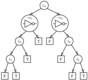
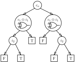
The tree shown in Fig. 5 has eight leaf-nodes and this is the value returned by the EVALUATE function in Alg. 1. After computing the quality of the tree shown in Fig. 5, CDE, tries all other possible components. For example, after a few attempts, CDE tries connecting a XOR gate to the primary inputs ci and i1. The resulting truth table is shown in Table 3.
| ci | i1 | ci ⊕ i1 | i2 | co | Σ |
|---|---|---|---|---|---|
| False True False True False True False True | False False True True False False True True | False True True False False True True False | False False False False True True True True | False False False True False True True True | False True True False True False False True |
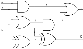
Clearly, the quality of the second tree, shown in Fig. 6, and having 6 leaf-nodes is better than the first one (with 8 nodes), hence the XOR gate is preferred. The process continues until the resulting decision tree has only a root and leaf nodes, i.e., it is a stump tree. The resulting functional decomposition for our running example is shown in 7. The difference, from the original design comes from the fact that we run CDE separately for each primary output and then we combine the resulting Boolean functions. Despite that the design is very similar to the original and exhaustive checking verifies that the implemented Boolean function is equivalent to that of the original full-adder.
We next extend the results from running CDE on the fulladder to a benchmark of Boolean functions.
6 Experimental Results
We have implemented CDE in Python using the Orange data mining and machine learning software suite [Curk et al., 2005] for inducing the binary decision trees. We have run all our experiments on a recent Linux platform based on a 2.8 GHz Intel i7 CPU and equipped with 4 GB of RAM.
6.1 Benchmark
We evaluate the performance of CDE on a benchmark of combinational circuits (see Table 4). The function decomposition benchmark contains small circuits and the 74XXX series functions which are manually decomposed by Hansen et al. [Hansen et al., 1999].
6.2 Experimental Results
CDE computed decompositions for 13 out of 15 benchmark instances. The algorithm could not compute decompositions for MUL3 and 74181 within the preallocated time quota of 15 min. In all successful cases the returned Boolean functions were logically equivalent to the target function.
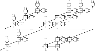
CDE produces interesting results in generating functions that do not only result in all metrics equal to 1 but also being equivalent (having equivalent system descriptions). This is the case for the instances HA, SUB1, PAR4 and PAR6. The design of the full subtractor is shown in Fig. 8 while Fig. 9 shows a scalable n-bit adder.
The main results of CDE are summarized in Table 5. The second and third column of Table 5 show the number of nodes and edges, respectively, of the system description returned by Alg. 1. The ratio of these sizes to the original graph sizes shown in Table 4 are given in the forth and fifth columns of Table 5. We can see that these values are often close to 1 which means that the graphs are of similar size. The rightmost column of Table 5 shows the time in seconds it takes for CDE to decompose the target Boolean function.
| name | |V | | |E| | |PI| | |PO| |
|---|---|---|---|---|
| HA | 6 | 4 | 2 | 2 |
| FA1 | 10 | 8 | 3 | 2 |
| FA2 | 15 | 9 | 5 | 3 |
| FA4 | 23 | 15 | 9 | 5 |
| SUB1 | 12 | 10 | 3 | 2 |
| MUX4 | 16 | 15 | 6 | 1 |
| DEMUX4 | 15 | 11 | 3 | 4 |
| MUL2 | 16 | 12 | 4 | 4 |
| MUL3 | 32 | 27 | 6 | 6 |
| PAR4 | 8 | 7 | 4 | 1 |
| PAR6 | 12 | 11 | 6 | 1 |
| 74182 | 33 | 28 | 9 | 5 |
| 74L85 | 47 | 44 | 11 | 3 |
| 74283 | 50 | 45 | 9 | 5 |
| 74181 | 87 | 79 | 14 | 8 |
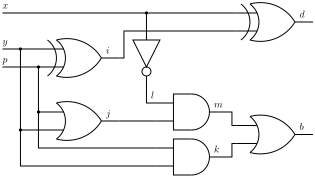
Table 6 shows the distribution of the components and the target and synthesized system descriptions. In general there are many complete functional sets and the choice of CDE is driven by, e.g., the ordering in the component library when breaking ties due to equivalent quality of the Boolean decision tree. Because of this potential equivalence of component library and gates, CDE may replace, for example, NAND components with OR components and inverters. The results in Table 6 show that the performance of CDE decreases with increasing the size of the target Boolean function. The ratios shown in this table are 1 if there is a 1:1 equivalence in gate numbers between the original circuit and the synthesized circuit; ratios less than 1 indicate that the synthesized circuit has more of that gate type than the original circuit.
a1 b1
| name | |V ′ | | |E′ | | |V |/|V ′ | | |E|/|E′ | | time [s] |
|---|---|---|---|---|---|
| HA | 6 | 4 | 1 | 1 | 0.59 |
| FA1 | 11 | 9 | 0.91 | 0 | 0.64 |
| FA2 | 23 | 20 | 0.65 | 0 | 3.17 |
| FA4 | 49 | 36 | 0.47 | 0 | 119.09 |
| SUB1 | 12 | 10 | 1 | 1 | 0.66 |
| MUX4 | 19 | 18 | 0.84 | 0 | 11.91 |
| DEMUX4 | 17 | 13 | 0.88 | 0 | 1.23 |
| MUL2 | 19 | 15 | 0.84 | 0 | 1.32 |
| MUL3 | - | - | - | - | - |
| PAR4 | 8 | 7 | 1 | 1 | 0.35 |
| PAR6 | 12 | 11 | 1 | 1 | 0.92 |
| 74182 | 52 | 47 | 0.63 | 0 | 36.36 |
| 74L85 | 90 | 87 | 0.52 | 0 | 532.20 |
| 74283 | 108 | 103 | 0.46 | 0 | 135.17 |
| 74181 | - | - | - | - | - |
| name | inverters | XOR | AND | OR |
|---|---|---|---|---|
| HA | - | 1 | 1 | - |
| FA1 | - | 1 | 1 | 0.5 |
| FA2 | - | 1 | 0.67 | 0.4 |
| FA4 | - | 0.22 | 0.27 | 0.24 |
| SUB1 | 1 | 1 | 1 | 1 |
| MUX4 | 2 | 0 | 0.8 | 0.33 |
| DEMUX4 | 1.33 | - | 1 | 0 |
| MUL2 | 0 | 2 | 1 | 0 |
| MUL3 | - | - | - | - |
| PAR4 | - | 1 | - | - |
| PAR6 | - | 1 | - | - |
| 74182 | 0.06 | - | 1.18 | 0.18 |
| 74L85 | 0.29 | 0 | 1.27 | 0.08 |
| 74283 | 0.55 | 0.29 | 0.4 | 0 |
| 74181 | - | - | - | - |
7 Conclusions
This work is introductory in a sense that, to the best of our knowledge, there is no in-depth algorithmic analysis of the problem of logic synthesis. As a future work we plan (1) to improve the CDE algorithm, (2) to formulate more problems related to logic synthesis, (3) to identify and implement more metrics for evaluating the performance of algorithms. Problems related to the problem of circuit synthesis is counting the number of decompositions and multi-parameter optimization of decompositions. Finally, metrics that can improve our evaluation include identification of maximal isomorphic subgraphs and similar.
Given the simplicity of our approach, it shows promise given that there are many optimizations that can be introduced. Such optimizations include better objective functions, applying heuristics to the simple greedy method, and learning sub-function component models that can be quickly substituted during the decomposition process.
@inproceedings{ijcai2013p243,
  title     = {Machine-Learning-Based Circuit Synthesis},
  author    = {Rokach, Lior and Kalech, Meir and Provan, Gregory M. and Feldman, Alexander},
  booktitle = {Proceedings of the Twenty-Third International Joint Conference on
               Artificial Intelligence, {IJCAI-13}},
  publisher = {AAAI Press / International Joint Conferences on Artificial Intelligence},
  editor    = {Francesca Rossi},
  pages     = {1635--1640},
  year      = {2013},
  month     = {8},
  url       = {https://ijcai.org/proceedings/2013/243},
}
TY - CPAPER TI - Machine-Learning-Based Circuit Synthesis AU - Rokach, Lior AU - Kalech, Meir AU - Provan, Gregory M. AU - Feldman, Alexander T2 - Proceedings of the Twenty-Third International Joint Conference on Artificial Intelligence, IJCAI-13 PB - AAAI Press / International Joint Conferences on Artificial Intelligence PY - 2013 SP - 1635 EP - 1640 UR - https://ijcai.org/proceedings/2013/243 ER -Copied
Machine-readable versions of this paper, for tools and AI agents:





