
Locality-Constrained Concept Factorization
Proceedings of the Twenty-Second International Joint Conference on Artificial Intelligence. Pages 1378-1382.
https://doi.org/10.5591/978-1-57735-516-8/IJCAI11-233
© 2011 International Joint Conferences on Artificial Intelligence
Abstract
Matrix factorization based techniques, such as nonnegative matrix factorization (NMF) and concept factorization (CF), have attracted great attention in dimension reduction and data clustering. Both of them are linear learning problems and lead to a sparse representation of the data. However, the sparsity obtained by these methods does not always satisfy locality conditions, thus the obtained data representation is not the best. This paper introduces a locality-constrained concept factorization method which imposes a locality constraint onto the traditional concept factorization. By requiring the concepts (basis vectors) to be as close to the original data points as possible, each data can be represented by a linear combination of only a few basis concepts. Thus our method is able to achieve sparsity and locality at the same time. We demonstrate the effectiveness of this novel algorithm through a set of evaluations on real world applications.
- [Cai et al., 2011] Deng Cai, Xiaofei He, and Jiawei Han. Lo- cally consistent concept factorization for document clus- tering. IEEE Transactions on Knowledge and Data Engi- neering, doi: 10.1109/TKDE.2010.165, 2011. DOI
- [He and Niyogi, 2003] Xiaofei He and Partha Niyogi. Lo- cality preserving projections. In Advances in Neural In- formation Processing Systems 16. 2003.
- [He et al., 2005] Xiaofei He, Shuicheng Yan, Yuxiao Hu, Partha Niyogi, and Hong-Jiang Zhang. Face recognition using laplacianfaces. IEEE Transactions on Pattern Anal- ysis and Machine Intelligence, 27(3):328-340, 2005.
- [Hoyer, 2004] Patrik O. Hoyer. Non-negative matrix factor- ization with sparseness constraints. Journal of Machine Learning Research, 5:1457-1469, December 2004.
- [Lee and Seung, 1999] Daniel D. Lee and H. Sebastian Se- ung. Learning the parts of objects by non-negative matrix factorization. In Nature, pages 788-791, 1999.
- [Lee and Seung, 2001] Daniel D. Lee and H. Sebastian Se- ung. Algorithms for non-negative matrix factorization. In NIPS, 2001.
- [Lee et al., 2007] H. Lee, A. Battle, R. Raina, and A.Y. Ng. Efficient sparse coding algorithms. In NIPS, 2007.
- [Xu and Gong, 2004] Wei Xu and Yihong Gong. Document clustering by concept factorization. In Proc. 2004 Annual ACM SIGIR Conference, 2004.
- [Yu et al., 2009] Kai Yu, Tong Zhang, and Yihong Gong. Nonlinear learning using local coordinate coding. In Ad- vances in Neural Information Processing Systems, 2009.
References were extracted automatically from the PDF and may contain errors.
Full text extracted automatically from the PDF; figures, tables and equations may differ. The PDF is the version of record.
1 Introduction
Data representation is a fundamental problem in many real world applications such as pattern recognition, computer vision, image clustering etc. Especially linear data representations, such as principal component analysis (PCA), locality preserving projection (LPP) [He and Niyogi, 2003; He et al., 2005], independent component analysis (ICA), nonnegative matrix factorization (NMF) [Lee and Seung, 1999] and concept factorization (CF) [Xu and Gong, 2004], have been widely used in these data analysis tasks.
Matrix factorization has been frequently used in linear data representation. Given a data matrix X, the above algorithms aim to find two or more matrix factors whose product is a good approximation to the original matrix. One factor consists of a set of new basis vectors which reveals the latent semantic structure, and the other factor can be considered as the coefficients (also referred as encodings) where each data point is a linear combination of the found bases. In real applications, the dimension of the new basis vectors is usually much smaller than that of the original data matrix. This gives rise to a compact representation of the data points which can facilitate other learning tasks such as clustering and classification.
NMF and CF have attracted great attention as efficient matrix decomposition methods. NMF aims to decompose a data matrix X into two matrix factors U and V so that UV provides a good approximation to X. The CF model is a variation of NMF in that each cluster is expressed by a linear combination of the data points and each data point is represented by a linear combination of the cluster centers. The major advantage of CF over NMF is that the NMF algorithm can only be performed in the original feature space of the data points, but the CF method can be performed on any data representation space, so that it can be kernelized and the powerful idea of the kernel method can be applied [Xu and Gong, 2004].
Since the dimension of the decomposed factors is much smaller than that of the original matrix, both NMF and CF map the data from high dimensional space to a low dimensional representation and obtain a sparse encoding of the data. However, the sparsity obtained by these methods does not always satisfy locality conditions. Since the local points share the greatest similarity, it would be more natural to represent the basis vectors using a few nearby anchor points, which leads to a more efficient representation of the data.
Recently, Cai et al. [Cai et al., 2011] proposed a Locally Consistent Concept Factorization approach to encode the geometrical information of the data space, which can extract the document concepts with respect to the intrinsic manifold structure. This method is able to discover the local geometrical structure, but does not always satisfy the locality conditions as we mentioned before. As to add sparseness constraint to the matrix factorization, Hoyer [Hoyer, 2004] showed how explicitly incorporating the notion of 'sparseness' improves the found decompositions. However, there is no work that includes locality and sparsity constraints at the same time to the best of our knowledge.
In this paper, we introduce a novel matrix factorization algorithm, called Locality-constrained Concept Factorization (LCF) which imposes a locality constraint onto the traditional concept factorization. By requiring the concepts (basis vectors) to be as close to the original data points as possible, each data can be represented by a linear combination of only a few nearby basis concepts, thus achieving sparsity and locality at the same time.
To achieve this goal, we incorporate the idea of Local Coordinate Coding [Yu et al., 2009] into the original objective function of concept factorization. And we also propose a multiplicative algorithm to efficiently solve the corresponding optimization problem.
2 Background
Factorization of matrices is generally non-unique, and a number of different methods of doing so have been developed by incorporating different constraints.
Suppose we have n data points {xi}ni=1 . Each data point xi ∈ Rm is m-dimensional and is represented by a vector. The vectors are placed in the columns and the whole data set is represented by a matrix X = [x1, · · · , xn] ∈ Rm×n. NMF aims to find an m × k matrix U and a k × n matrix V where the product of these two factors is an approximation to the original matrix, represented as X ≈ UV. Each column vector of U, ui, can be regarded as a basis and each data point xi is approximated by a linear combination of these k bases, weighted by the components of V: xi ≈ ∑kj=1 ujvji.
The speciality of NMF is that it enforces that all entries of the factor matrices must be non-negative. One limitation of NMF is that the non-negative requirement is not applicable to applications where the data involves negative number. The second is that it is not clear how to effectively perform NMF in the transformed data space so that the powerful kernel method can be applied.
Concept Factorization is proposed striving to address the above problems while inheriting all the strengths of the NMF method. In the CF model, we rewrite the NMF model by representing each base (cluster center) uj by a linear combination of the data points uj = ∑i wijxi where wij ≥ 0. Let W = [wij ] ∈ Rn×k , CF tries to decompose the data matrix satisfied the following condition
Using the Frobenius norm to qualify the approximation, CF tries to minimize the following objective function
3 Locality-constrained Concept Factorization
In this section, we introduce our Locality-constrained Concept Factorization (LCF) algorithm, which takes the locality constraint as an additional requirement. The algorithm presented in this paper is fundamentally motivated from the concept of local coordinate coding [Yu et al., 2009].
3.1 The Objective Function
First we introduce the concept of coordinate coding.
Definition A coordinate coding is a pair (γ, C), where C ⊂ Rd is a set of anchor points, and γ is a map of x ∈ Rd to [γv(x)]v∈C ∈ R|C| such that ∑v γv(x) = 1. It induces the following physical approximation of x in Rd : γ(x) = ∑v∈C γv(x)v.
According to this definition, the CF model can be considered as a coordinate coding where the basis vectors uj = ∑i wijxi are a set of anchor points, and each column of V
contains the coordinates for each data point with respect to the anchor points. In order to add the local sparse constraint to the traditional concept factorization, we require that each original data point should be sufficiently close to only a few anchor points. This can be achieved by introducing the following term to measure the locality and sparsity penalty:
The above constraint incurs a heavy penalty if xi is far away from the anchor point uj while its coordinate vji with respect to uj is large. Therefore, by minimizing R, we essentially try to formalize our intuition that xi is close to the anchor points uj as much as possible, otherwise its coordinate with respect to uj tends to be zero.
With the locality constraint, our LCF algorithm reduces to minimize the following objective function:
with the constraint that W and V are non-negative matrices. The λ ≥ 0 is a regularization parameter.
3.2 The Algorithm
We introduce an iterative algorithm to find a local minimum for the optimization problem. The objective function can be rewritten as follows:
where Di = diag(|vi|) ∈ RK×K . Using the matrix property Tr(AB) = Tr(BA), ‖A‖2 = Tr(AT A) and Tr(A) = Tr(AT ), we have
Let ψjk and φki be the Langrange multiplier for constraints wjk ≥ 0 and vki ≥ 0, respectively. We define matrix Ψ =
[ψjk] and Φ = [φki], then the Langrange L is
Define K = XT X, define a column vector a = diag(K) ∈ RN . Let A = (a, · · · , a)T be a K ×N matrix whose rows are aT . Define a column vector b = diag(WT KW) ∈ RK . Let B = (b, · · · , b) be a K × N matrix whose columns are b. The partial derivatives of L with respect to W and V are:
Using the Karush-Kuhn-Tucker conditions (also known as the KKT conditions) ψjkwjk = 0 and φkivki = 0, we get the following equations:
The above equations lead to the following update rules:
We have the following theorem regarding the above iterative updating rules. Theorem 1 guarantees the convergence of the iterations in Eq. (4) and (5) and therefore the final solution will be a local optimum.
Theorem 1. The objective function O in Eq. (2) is nonincreasing under the update rules in Eq. (4) and Eq. (5). The objective function is invariant under these updates if and only if W and V are at a stationary point.
To prove Theorem 1, we use an auxiliary function similar to that used in the Expectation-Maximization algorithm.To make the proof complete, we restate the definition of auxiliary function and its property which will be used to prove the algorithm convergence.
Definition G(x, x′ ) is an auxiliary function for F(x) if the conditions
are satisfied.
Lemma 2. If G is an auxiliary function, then F is nonincreasing under the update
The equality F(xt+1 ) = F(xt ) holds only if xt is a local minimum of G(x, xt ). By iterating the updates in Eq. (6), the sequence of estimates will converge to a local minimum xmin = argminx F(x). Next, we will define an auxiliary function for our objective function and use Lemma 2 to show that the minimum of the objective function is exactly our update rule, thereby Theorem 1 is proved.
First, we prove the convergence of the update rule in Eq. (4). Considering any element wab in W, we use Fwab to denote the part of O which is only relevant to wab. Since the update is essentially element-wise, it is sufficient to show that each Fwab is nonincreasing under the update step of (4). We prove this by defining the auxiliary function G for Fwab as follows.
Lemma 3. The function
is an auxiliary function for Fwab , the part of O which is only relevant to wab.
Proof. Since G(w,w) = Fwab (w) is obvious, we only need to show that G(w, w(t) ab ) ≥ Fwab (w). To do this, we compare G(w, w(t) ab ) with the Taylor series expansion of Fwab (w):
Since
and
Then we define an auxiliary function for the update rule in Eq. (5). Similarly, let Fvab denote the part of O relevant to vab. Then the auxiliary function regarding vab is defined as follows.
Lemma 4. Function
is an auxiliary function for Fvab , the part of O which is only relevant to vab.
The proof is essentially similar to the proof of Lemma 3 and is omitted here due to space limitation. With the above lemmas, now we give the proof of Theorem 1.
Proof of Theorem 1: From Lemma 3 we know that G(w, w(t) ab ) is an auxiliary function for Fwab , and from Lemma 4 we know that G(v, v(t) ab ) is an auxiliary function for Fvab . According to Lemma 2, by solving w(t+1) = arg minw G(w, w(t) ab ), We obtain
and by solving v(t+1) = arg minz G(v, v(t) ab ), We obtain
which are exactly the same updates as in Eq. (4) and (5). Therefore, the objective function O in Eq. (2) is nonincreasing under these updates. □
4 Experiments
In this section, we show the data clustering performance of the proposed method, and compare the results with four other related methods using the same data set. The algorithms that we evaluated are listed below:
- Traditional K-means (Kmeans).
- Nonnegative Matrix Factorization (NMF) [Lee and Seung, 2001].
- Concept Factorization (CF) [Xu and Gong, 2004].
- Non-negative Matrix Factorization with Sparseness Constraints (SparseNMF) [Hoyer, 2004].
- Our proposed Locality-constrained concept Factorization (LCF).
We use two metrics to evaluate the clustering performance. One metric is accuracy (AC), which is used to measure the percentage of correct labels obtained. The second metric is the normalized mutual information (̂ MI). In clustering applications, mutual information is used to measure how similar two sets of clusters are. The definitions of these two metrics can be found in [Xu and Gong, 2004]. The performance is evaluated by comparing the cluster label of each sample with the label provided by the data set.
| dataset | size(N) | dimensionality(M) | of classes(K) |
| Yale | 165 | 1024 | 15 |
| ORL | 400 | 1024 | 40 |
The evaluations were conducted for the cluster numbers ranging from 2 to 10. For each given cluster number k, we randomly chose k clusters and ran the test 10 times, and the final scores were obtained by calculating the average and variance over the 10 test runs. Since the evaluated methods whose clustering results depend on the initialization, each test run consists of 10 sub-runs from which we chose the best result to report.
In the experiments, the parameters were set to be the values that each algorithm can achieve its best results. For our LCF algorithm, the regularization parameter is set to be λ = 0.3.
4.1 Data Sets
The experiments are conducted on two data sets. One is the Yale Database, and the other is Cambridge ORL face database. The important statistics of these data sets are described below (also summarized in Table 1):
- The Yale database contains 165 gray scale images of 15 individuals. All images demonstrate variations in lighting condition (left-light, center-light,right-light), facial expression (normal, happy, sad, sleepy, surprised and wink), and with/without glasses.
- The ORL database contains ten different images of each of 40 distinct subjects, thus 400 images in total. For some subjects, the images were taken at different times, varying the lighting, facial expressions (open/closed eyes, smiling/not smiling) and facial details (glasses/no glasses). All the images were taken against a dark homogeneous background with the subjects in an upright, frontal position (with tolerance for some side movement).
In all the experiments, images are preprocessed so that faces are located. Original images are first normalized in scale and orientation such that the two eyes are aligned at the same position. Then the facial areas were cropped into the final images for clustering. Each image is of 32 × 32 pixels with 256 gray levels per pixel.
4.2 Clustering Results
Fig. 1 and 2 show the plots of accuracy and normalized mutual information versus the number of clusters for different algorithms on the Yale dataset. As can be seen, our proposed LCF algorithm consistently outperforms all the other algorithms. The detailed clustering results are shown in Table 2. The last row shows the average accuracy (normalized mutual information) over k. Comparing to the best algorithm other than our proposed LCF i.e. SparseNMF, our algorithm LCF achieves 4.41% improvement in accuracy and 5.69% improvement in normalized mutual information.
| k | Kmeans | NMF | CF | SparseNMF | LCF |
|---|---|---|---|---|---|
| Accuracy(%) | |||||
| 2 | 78.18 ± 16.86 | 73.18 ± 18.00 | 71.82 ± 20.21 79.09 | ± 17.51 | 85.00±17.01 |
| 3 59.09 ± | 12.14 62.73 ± | 11.42 | 58.79 ± 9.70 | 63.33 ± 9.91 | 76.36±17.29 |
| 4 51.36 | ± 7.20 56.14 ± | 5.75 | 53.18 ± 9.55 | 56.82 ± 7.87 | 58.64±9.52 |
| 5 50.36 | ± 3.36 52.55 ± | 5.30 | 52.36 ± 5.74 | 54.18 ± 6.94 | 58.18±7.18 |
| 6 46.52 | ± 6.85 49.55 ± | 8.91 | 48.18 ± 8.10 | 51.06 ± 8.63 | 52.42±10.74 |
| 7 43.25 | ± 6.42 46.49 ± 5.97 | 47.14 ± 5.92 | 47.66 ± 5.29 | 49.48±4.84 | |
| 8 44.20 | ± 3.78 | 45.00 ± 3.56 | 46.36 ± 2.91 | 47.05 ± 2.84 | 49.43±5.69 |
| 9 43.74 | ± 7.03 43.23 ± | 4.33 | 44.65 ± 6.32 | 42.32 ± 4.50 | 47.68±5.71 |
| 10 | 39.45 ± 4.49 | 41.36 ± 5.77 | 43.91 ± 5.19 | 41.00 ± 3.34 | 45.00±7.50 |
| Avg. | 50.68 ± 7.57 | 52.25 ± 7.67 | 51.82 ± 8.18 | 53.61 ± 7.43 | 58.02±9.50 |
| NormalizedMutual Information(%) | |||||
| 2 40.58 ± | 39.97 32.53 ± 38.16 | 34.66 ± | 43.79 | 42.85 ± 40.46 | 56.78±39.45 |
| 3 | 38.49 ± 20.50 | 34.28 ± 16.27 | 31.99 ± 20.51 | 32.70 ± 15.86 | 54.24±30.02 |
| 4 | 31.00 ± 6.92 | 32.78 ± 9.04 | 31.48 ± 11.96 | 35.88 ± 10.04 | 36.13±9.92 |
| 5 | 39.08 ± 7.99 | 40.11 ± 8.46 | 38.13 ± 8.51 | 40.21 ± 7.76 | 42.91±10.41 |
| 6 | 40.03 ± 11.26 | 37.74 ± 10.81 | 38.99 ± 11.40 | 39.83 ± 11.50 | 42.43±11.94 |
| 7 | 36.39 ± 6.24 | 36.89 ± 6.36 | 40.46 ± 5.32 | 40.73 ± 5.37 | 42.41±4.47 |
| 8 | 40.78 ± 4.09 | 41.07 ± 3.64 | 40.48 ± 2.26 | 40.90 ± 3.08 | 43.78±3.70 |
| 9 | 41.58 ± 7.28 | 40.94 ± 5.24 | 40.90 ± 7.06 | 40.86 ± 3.54 | 43.12±5.09 |
| 10 | 39.04 ± 5.58 | 39.83 ± 4.59 | 41.85 ± 4.96 | 41.07 ± 2.63 | 44.45±7.32 |
| Avg. | 38.55 ± 12.20 | 37.35 ± 11.40 | 37.66 ± 12.86 | 39.45 ± 11.14 | 45.14±13.59 |
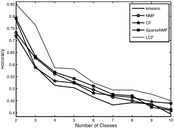
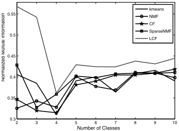
Fig. 3 and Fig. 4 show the graphical clustering results for the ORL data set. LCF obtains the best result for most of the cases. SparseNMF fails to consider the locality condition, and in some cases performs even worse than Kmeans. Table 3 shows the detailed clustering accuracy and normalized mutual information. Comparing to the best algorithm other than our proposed LCF algorithm, i.e., SparseNMF, LCF achieves
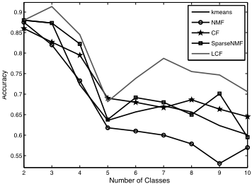
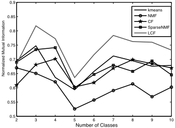
5.8% improvement in accuracy. For normalized mutual information, LCF achieves 6.4% improvement.
4.3 Learning the Overcomplete Basis
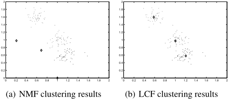
Usually, matrix factorization methods are used for dimension reduction in many applications. However, [Lee et al., 2007] shows that in some cases, it is desirable to learn the overcomplete basis. Here we evaluate the performance of our algorithm in this aspect. To show the performance for learing the overcomplete basis of our proposed algorithm, 150 data points from mixture of three Gaussians in a 2- dimensional space are randomly generated. NMF and LCF are conducted to obtain three basis vectors and cluster these data points into 3 clusters. Fig 5 shows that our LCF obtains better results than NMF. The bases obtained by NMF are far away from the original points. However, since we add a locality constraint, the three bases obtained by LCF exactly reside in the cluster centers, which leads to a better data representation.
| k | Kmeans NMF | CF | SparseNMF | LCF |
|---|---|---|---|---|
| Accuracy(%) | ||||
| 2 88.00 ± 17.64 | 87.50 ± 17.64 | 86.00 ± 16.09 | 88.00 ± 17.49 | 88.00±17.78 |
| 3 87.33 ± 10.73 | 82.00 ± 11.27 | 82.67 ± 12.36 | 87.33 ± 10.93 | 91.33±9.80 |
| 4 72.25 ± 13.53 | 73.25 ± 8.37 | 79.50 ± 9.34 | 82.25 ± 7.94 | 84.50±9.92 |
| 5 63.60 ± 11.62 | 61.80 ± 7.40 | 69.00±8.26 | 63.80 ± 7.77 | 68.20 ± 8.27 |
| 6 65.67 ± 7.04 | 61.00 ± 7.57 | 68.00 ± 7.74 | 69.17 ± 5.83 | 73.83±6.99 |
| 7 67.14 ± 13.19 | 60.00 ± 6.23 | 66.71 ± 7.06 | 68.00 ± 6.07 | 78.71±11.00 |
| 8 65.63 ± 7.57 | 57.88 ± 5.76 | 68.63 ± 6.29 | 65.00 ± 6.98 | 75.50±6.20 |
| 9 62.33 ± 7.44 | 53.11 ± 4.55 | 66.33 ± 7.32 | 70.11 ± 6.35 | 74.67±8.18 |
| 10 60.10 ± 7.23 | 57.00 ± 6.15 | 64.50 ± 6.17 | 59.50 ± 7.79 | 70.60±6.62 |
| Avg. 70.23 ± 10.66 | 65.95 ± 8.33 | 72.37 ± 8.96 | 72.57 ± 8.57 | 78.37±9.42 |
| NormalizedMutual Information(%) | ||||
| 2 69.45±42.12 | 67.02 ± 40.95 | 60.95 ± 40.11 | 68.99 ± 42.71 | 68.38 ± 41.04 |
| 3 74.75 ± 17.48 | 65.08 ± 15.94 | 68.11 ± 18.03 | 73.43 ± 17.50 | 81.76±17.12 |
| 4 63.64 ± 16.27 | 62.09 ± 9.01 | 70.15 ± 11.54 | 74.12 ± 9.17 | 77.26±13.09 |
| 5 59.30 ± 12.75 | 52.59 ± 9.10 | 60.30 ± 8.93 | 60.03 ± 9.42 | 63.61±10.83 |
| 6 65.75 ± 6.22 | 55.72 ± 5.45 | 61.83 ± 7.03 | 64.70 ± 7.13 | 71.63±8.32 |
| 7 71.19 ± 10.56 | 59.06 ± 6.53 | 66.86 ± 7.62 | 67.92 ± 7.45 | 78.39±10.46 |
| 8 69.48 ± 6.22 | 61.38 ± 4.54 | 69.89 ± 4.74 | 65.77 ± 5.71 | 76.23±5.03 |
| 9 67.56 ± 7.50 | 56.88 ± 5.32 | 68.47 ± 5.68 | 69.42 ± 5.19 | 76.01±7.92 |
| 10 67.89 ± 6.54 | 60.23 ± 6.54 | 66.96 ± 5.40 | 64.55 ± 6.59 | 73.25±6.10 |
| Avg. 67.67 ± 13.96 | 60.01 ± 11.49 | 65.95 ± 12.12 | 67.66 ± 12.32 | 74.06±13.32 |
5 Conclusions
In this paper we proposed a novel matrix factorization method, called Locality-constrained Concept Factorization (LCF). This method enforces a locality constraint onto the traditional concept factorization. By requiring the concepts (basis vectors) to be as close to the original data points as possible, each data can be represented by a linear combination of only a few nearby basis concepts, thus achieving sparsity and locality at the same time. The experimental results on two standard face databases have demonstrated the effectiveness of our approach over other matrix factorization techniques, especially for the data clustering applications.
Acknowledgments
This work was supported by the Fundamental Research Funds for the Central Universities under grant 2009QNA5024.
@inproceedings{ijcai2011p233,
  title     = {Locality-Constrained Concept Factorization},
  author    = {Liu, Haifeng and Yang, Zheng and Wu, Zhaohui},
  booktitle = {Proceedings of the Twenty-Second International Joint Conference on
               Artificial Intelligence, {IJCAI-11}},
  publisher = {AAAI Press/International Joint Conferences on Artificial Intelligence},
  editor    = {Toby Walsh},
  pages     = {1378--1382},
  year      = {2011},
  month     = {7},
  doi       = {10.5591/978-1-57735-516-8/IJCAI11-233},
  url       = {https://doi.org/10.5591/978-1-57735-516-8/IJCAI11-233},
}
TY - CPAPER TI - Locality-Constrained Concept Factorization AU - Liu, Haifeng AU - Yang, Zheng AU - Wu, Zhaohui T2 - Proceedings of the Twenty-Second International Joint Conference on Artificial Intelligence, IJCAI-11 PB - AAAI Press/International Joint Conferences on Artificial Intelligence PY - 2011 SP - 1378 EP - 1382 DO - 10.5591/978-1-57735-516-8/IJCAI11-233 UR - https://doi.org/10.5591/978-1-57735-516-8/IJCAI11-233 ER -Copied
Machine-readable versions of this paper, for tools and AI agents:





