Cluster Indicator Decomposition for Efficient Matrix Factorization

1 Introduction

Many machine learning applications require processing large amounts of high dimensional data. In these applications, the data are represented as a m×nmatrix X, e.g. images, videos, kernel matrices, spectral graph. As data size and the amount of redundancy increase fast with dimensionality m and n, it is desirable to obtain compact and concise representations of X to make data analysis and interpretation easier, e.g., a lowrank approximation of original data.

Low-rank approximation of matrices have been widely used in broad artificial intelligence applications such as image denoising and compression [Zhang et al., 2009], face recognition [Turk and Pentland, 1991], motion scene reconstruction [Han and Kanade, 2001], scene appearance approximation [Garg et al., 2009], and part of objects representation [Lee and Seung, 1999] etc. Among them, kernel matrix approximation is one of the most important applications. Kernel methods play a central role to successfully model computer vision data with highly complex, nonlinear structures, e.g. support vector machine, kernel Fisher discriminant analysis, and kernel principal component analysis. But the computational complexities of large kernel matrices in terms of both space (quadratic) and time (usually cubic) are quite challenge in practical applications. Low-rank approximations of the kernel matrix can effectively tackle large-scale datasets with no significant decrease in performance [Williams and Seeger, 2000; Zhang et al., 2008; Fowlkes et al., 2004; Talwalkar et al., 2008].

There are a very large number of different low rank approximation methods [Bach and Jordan, 2005; Frieze et al., 2004], among them Singular Value Decomposition (SVD) is the best known and most widely used one, because it provides the best low rank approximation so far and can be readily computed.

Another popular low-rank approximation algorithm is Nystr¨om decompositions, because it is easy to be computed and also the vectors involved in factorization are "interpretable". Nystr¨om style decompositions have been widely used to speed up the computation of large kernel matrix [Williams and Seeger, 2000; Zhang et al., 2008; Drineas and Kannan, 2003; Fowlkes et al., 2004; Srebro and Jaakkola, 2003].

In this paper, we propose a new clustering based low-rank matrix approximation. This decomposition uses cluster indicators which have a nice property that they can be stored into a single vector, while provide the approximation capability of rank-K approximation. This Cluster Indicator Decomposition (CID) is thus compact (comparable and even more compact than SVD). Meantime, it is also interpretable because the basis vectors are cluster indicators.

The clustering model here also naturally suggests a Relaxed Cluster Indicator Decomposition where the nonzero elements of cluster indicators are not forced to be "1". Our new low-rank matrix approximation methods have close connection to Nystr¨om style decompositions and several other closely related variants. But our methods have much better approximation accuracy than related approaches. Using four standard image datasets, we evaluate the performance of our methods by image compression and kernel matrix approximation applications in term of reconstruction errors and classification accuracy. We provide a new insight to low-rank matrix approximation and our methods can be widely applied into many computer vision applications.

2 Cluster Indicator Decomposition (CID)

For any rectangular (or non-symmetric square) input matrix X ∈ ℜm×n, we seek the CID decomposition of X as

In addition, each row of F has exactly one nonzero element "1". Thus F = (f1, · · · , fk1 ) is the cluster indicator matrix for row clustering of X, i.e., the non-zeros of fp indicate rows of X which form a row cluster Rp. Similarly, G = (g1, · · · , gk2 ) is the cluster indicator matrix for column clustering of X, where the non-zeros of gq indicate columns of X forming a column cluster Cq. The factors F, S,G are obtained by

which can be equivalently written as

This can be viewed as an extension of the standard "one-way" K-means clustering:

where μq is the centroid of cluster Cq . The simultaneous clustering of rows and columns of X can be viewed as block clustering and Spq is the "mean" of the block cluster.

Storage of CID

CID is very compact. The indicator matrix F can be stored in an m-vector fCID of b1-bit integers, where b1 = ⌈log2k1⌉ and fCID(j) indicate the index of row cluster that j-th row belongs to. Similarly, indicator matrix G can be stored in an n-vector gCID of b2-bit integers where b2 = ⌈log2k2⌉. (F,G) requires mb1 + nb2 bits storage, which is much less than 64(m+n) bits storage for a pair of singular vectors (ul, vl). For this reason, we sometimes call it rank-0 storage. S is stored as k1k2 real numbers. Thus the total storage Γ for CID in unit of 64-bit reals is

We note that for SVD truncated into KSV D terms, the storage is ΓSVD = KSV D(m+n). A very simple implementation uses a whole 64-bit integer for F and other 64-bit integer for G. This simple CID use storage less than SVD if

2.1 Relaxed CID

In CID, each row of F has exactly one nonzero element which is "1". We now relax this nonzero element to a real number. This improves the matrix approximations, but increase storage slightly. We can also relax G similarly. We call this decomposition as Relaxed CID.

Storage of Relaxed CID

Because each row of F has only one nonzero, the k1 columns of F = (f1, · · · , fk1 ) can be stored in a single mvector as fRCID Cluster labels of each row is stored in fCID (see storage of CID). Furthermore, because each element of fCID has only b1 = logk1 bits (for k1=32 clusters, b1 = 5), fCID can be packed in to the least significant b1-bits in fRCID's mantissa. G is stored similarly. Over-all, the storage of F,G is equivalent to storage of a pair singular vectors of SVD (we may call Relaxed CID as "CID with rank-1 storage").

2.2 Computational algorithm of RCID and CID

Optimization of Eq. (3) with discrete constraints of Eqs. (1,2) is an NP-hard combinatorial optimization. Here we use a continuous approach to first find a relaxed solution.

We do a transformation. Let ˜F = FD-1/2 f where Df = diag(m1, · · · ,mk1 ) andmp = |Rp| is the size of row-cluster Rp. Clearly, ˜FT ˜F = I where I is an identity matrix of appropriate size. Similarly, let ˜G = GD-1/2 g where Dg = diag(n1, · · · , nk2 ) and nq = |Cq| is the size of columncluster Cq. Clearly, ˜GT ˜G = I. Let ˜S = D1/2 f SD1/2 g be the new central factor.

It is obvious that ˜F˜S ˜GT = FSGT . But in terms of these new factors, the constraints become easier to deal with. Now, for notational simplicity, we use F for ˜F, G for ˜G, S for ˜S. These factors are obtained from the optimization

Since F is nonnegative, the orthogonality of F implies each row of F has only one nonzero. But this nonzero element is not restricted to "1", as required by a strict "cluster indicator". For this reason, we call F "relaxed" cluster indicator. Similarly, the relaxed indicator G is computed in this optimization. Therefore, this optimization gives solution for Relaxed CID.

Once the relaxed indicators are obtained in Relaxed CID, we set the non-zeros in F,G to "1" , fixing them, and update S to obtain the solution for CID.

Here we outline the algorithm [Ding et al., 2006] to solve the orthogonal tri-factorization Eq.(8). Here the data X is nonnegative. The algorithm is given as below:

( S0) Initialize G. Do K-means clustering on columns of X into k2 clusters. This gives cluster indicator G and let G0 = G+ 0.2. Normalize each column of G0 to 1 using L2-norm (thus GT0 G0 ∼= I). Initialize F in same way by clustering rows of X into k1 clusters.

( S1) Repeat until convergence:

Notice that the RHS factors (square brackets) of Eqs. (10) and (11) are not square rooted as in [Ding et al., 2006]. Thus algorithm here converges faster than that in [Ding et al., 2006]. The convergence of Eqs. (10) and (11) can be vigorously proved (details are skipped due to space limitation).

Real Life Image Compression

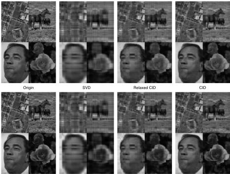
Fig. 1 shows the real images compression results using CID and Relaxed CID. The original image and SVD results are also shown. From the figures, we can see that CID compressed images are much more clear than SVD results. The image details are described in the first paragraph of §4.

2.3 Error bounds for CID

Let J ∗ CID be the optimal reconstruction error of CID and and J ∗ RCID be the optimal reconstruction error of relaxed CID. We show there exists an easily computable upper bound:

Theorem 2.1 In CIDand RCID compositions of the inputX, we have the upper bound

where J columns Kmeans (X), J rows Kmeans (Y) are obtained as following:

CID bound calculation. (1) Do K-means clustering on the columns of X. Let J columns Kmeans (X) be the corresponding objective function value. Let Y be the centroid data, i.e., each xi is replaced by its corresponding cluster centroid:

(here we assume, without loss of generality, that columns of X are ordered such that data points within same cluster are adjacent, and setting k1 = k2 = k to simplify the notation). (2) Do K-means clustering on rows of the m-by-n matrix Y.

This is identical to the clustering of the rows of the condensed centroid data Y:

Clustering on Y is faster since Y is size of m-by-k and k ≪ n. J rows Kmeans (Y) is the objective function value of this clustering.

Proof of Theorem 1. The inequality J ∗ RCID ≤ J ∗ CID is true because the relaxed indicator F,G from "1" improves the approximation. To obtain an upper bound of JCID, it is sufficient to find a feasible solution of the optimization of Eq. (3) or the equivalent block clustering formulation of Eq. (4). Clearly, the solution (F0,G0) obtained by the CID bound computing algorithm above is a feasible solution of the block clustering. Furthermore, the block clustering objective function value of the solution (F0,G0) is exactly JCID(F0,G0) = J columns Kmeans (X) + J rows Kmeans (Y). By definition, the optimal solution should have a lower objective comparing to a feasible solution, i.e., J ∗ CID ≤ JCID(F0, G0). ■

2.4 CID for symmetric/kernel matrices

For kernel (and generic symmetric) matricesW, due to symmetry, F = G. Therefore, the decomposition becomes

where G is restricted to be an indicator matrix. As discussed in §2.1,the relaxed indicator S and factor G are obtained from the optimization

The algorithm to compute G, S is very similar to that of §2.2. We outline the algorithm as following:

(B0) Initialize G by clustering rows of W.

(B2) Update G:

where Λ is the Lagrangian multiplier to enforce GT G = I.

Repeat (B1, B2) until convergence. We obtain Relaxed CID result. After that, we fix the nonzero elements of F,G to be 1, and update S to get CID result. Eq. (16) uses least square objective. A more sophisticated objective is using Laplacian formulism as presented in [Luo et al., 2009].

The above algorithm assumes the input data W is nonnegative. When W has mixed signs, S has mixed signs. We have algorithm for updating F,G, bS for this case. Details are skipped due to space limit.

The upper error bound of Theorem 1 can also be extended to this case. Because W is symmetric, only clustering of columns of W are done, which gives cluster indicator G0. Let YW be constructed same as Y in Theorem 1, and evaluate J rows Kmeans (YW) using the cluster indicator G0. We have

Theorem 2.2 In CID composition for input symmetric matrix W, we have the upper bound for CID decomposition W ∼= (G∗ )S∗ (G∗ )T

3 Reconstruction Complexity of CID

One important application of matrix decomposition is that it helps to solve large scale problems due to storage reduction. Here, the speed of reconstruction of Kernel becomes a critical factor because we have to reconstruct the kernel very frequently. For example, in SVMs for classification.

We note that reconstruction in CID is extremely fast, as compared to other decomposition methods such as Nystr¨om, SVD, CUR, etc. Specifically, we note that in CID, F is row cluster indicator and its role is to pick (index) the correct block means Skl. There is no computation involved. The reconstruction of CID approximation is (supposing X is a kernel matrix K),

where Ri is the row cluster that row index i belongs to, and Cj is the column cluster that column index j belongs to. We can obtain the kernel value by two indexing operations.

For other decomposition approaches, the reconstruction complexity is much higher. For example, in SVD approximation, Kij ≈ ∑p UipSppUjp requires 3KSVD floating point operations. For Nystr¨om, it is even higher.

In an efficient implementation of Support Vector Machines, chunking techniques are widely employed. In chunking, we compute (reconstruct) kernel values for a chunk of the kernel matrix, use them for some computation, and throw them away. For the same chunk of the kernel matrix, if we later need, we recompute them anew. This is repeated many times. This is extremely expensive for the traditional approaches. But for CID, we access the kernel matrix values as if all the entries have been already computed and been stored.

4 Experimental Results

4.1 Reconstruction errors of CID

Image Compression

In order to examine CID low-rank approximation schemes on rectangular data matrices, we use image compression application and compare results to SVD that is considered as the best low-rank approximation method so far. First, we illustrate four image compression results using SVD and CID in Fig. 1. These four images are randomly selected from three public image databases: two fromWANG's dataset [Wang et al., 2001], one from Google map, and one from Ferret face database [Philips et al., 1998]. In order to compare them together, all images are resized to 384×256. The parameters are selected to make them use the same storage for compressed images. For color images (top row of Fig. 1), all methods are done independently on red, green, and blue channels. The reconstruction (low-rank approximation) errors are defined as

‖X - ˜X‖2/‖X‖2, where X is the original image and ˜X is the reconstruction image). Compared to SVD, in Fig. 1, CID and Relaxed CID provide not only more interpretable decomposition, but also much better low-rank approximation.

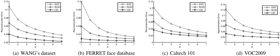
Besides the above illustrative demonstrations, we also systematically perform the image compression on four public computer vision datasets: WANG's dataset [Wang et al., 2001], FERRET face database [Philips et al., 1998], Caltech 101 [Perona et al., 2004], and PASCAL Visual Object Classes 2009 Challenge (VOC2009) 1 . The experimental setup is the same as the above descriptions. When the rank of SVD increase from 1 to 7, we select the corresponding parameters for CID and Relaxed CID to make them use the same storage for compressed images. The average image reconstruction errors of SVD, CID, and Relaxed CID are plotted in Fig. 2. Using the same storage, CID always has the best low-rank approximation, and Relaxed CID is also consistently more accurate than SVD. We note that CID outperforms other methods the more structure the better and the at the smaller storage (small KSVD) the better. On the other hand, for data without structure, CID does not outperform SVD.

Kernel Matrix Approximation To measure CID low-rank approximation schemes on symmetric/kernel matrices, we perform CID and Relaxed CID on 3 commonly used human face datasets: AT&T face dataset 2 (Dim=644, N=400), MNIST digit images [Cun et al., 1998] (Dim=784, N=150), and The Japanese Female Facial Expression (JAFFE) Database 3 ( Dim=4096, N=213), and one hand written digitletter image database: BinAlpha 4 (Dim=320, N=1404). We perform methods on Gaussian kernel K(x, y) = exp(-‖x - y‖2/γ 2 ) (it is the standard one to evaluate the low-rank approximation) where γ is the average of pairwise distances. We compare CID and Relaxed CID to SVD and major Nystr ¨om style decompositions on kernel matrices approximations. The results are shown in Fig. 3.

1 http://pascallin.ecs.soton.ac.uk/challenges/VOC/

2 http://www.cl.cam .ac.uk/research/dtg/attarchive/facedatabase.html

3 http://www.kasrl.org/jaffe.html

4 http://www.cs.toronto.edu/ roweis/data.html

For the Nystr¨om style decompositions, we run 20 random trials and obtain the average reconstruction errors. Four methods are compared in our experiments: (1) standard Nystr¨om (Nystrom), (2) Medoid method (Medoid) [Zhang et al., 2008], (3) Frieze et al.'s method [Frieze et al., 2004] (FKV), (4) CUR. When the rank K of SVD changes from 2 to 9, parameters in all other methods are selected to guarantee the same storage is used. Obviously, our CID and Relaxed CID methods have much better low-rank approximation than all other related methods.

4.2 Kernel matrix approximation in classification

We embed the decomposition into kernel classification machines to investigate the efficiency. We compare CID to SVD and Nystr¨om in terms of classification accuracy and kernel reconstruction time. We use RBF kernel Support Vector Machines (a modification of LIBSVM 5 ) with 10-fold cross validation. We determine the parameters as following. By running 10-fold cross validation with gaussian parameter γ = [2-10 ¯ r, 2-9 ¯ r, ..., 210 ¯ r], and C parameter C = [2-10 , 2-9, ..., 210 ] where ¯ r is the average Euclidean distance of all pairs of data points. Let (γopt, Copt ) denote the parameters which generate the best 10-fold cross validation results, then we perform decompositions on the kernel using gaussian parameter γopt: Kopt (i, j) = exp(-‖xi - xj ‖2/γ 2 opt ).

We chose k = 1, 4, 8 in our experiments. For Nystr ¨om and CID, we approximate the best kernel Kopt with the same size of storage as SVD. Notice that for CID, the kernel is reconstructed by using Eq. (18), which is extremely computationally simple.

We report results in Table 4.1. In LIBSVM, we use 1vs-1 scheme, and reported results are derived by summing up all the base binary classifiers over all the cross validation folds (except the accuracy is the average accuracy). In Table 4.1, results show that CID outperforms SVD and Nystr¨om in terms of both classification accuracy and kernel reconstruction CPU time. We also notice that in JAFFE dataset, even though we only use the same storage as k = 1 in SVD, the classification accuracy is still very high (96.64%), i.e. CID works well with very limited memory.

5 www.csie.ntu.edu.tw/ cjlin/libsvm/

5 Conclusion

We proposed a family of algorithms to derive effective lowrank matrix decompositions which are both accurate and highly interpretable. In CID, column/row matrix factors are cluster indicators which can be compacted into very small space and the middle factor is the block cluster mean. Furthermore, the reconstruction is extremely fast. We derived several error bounds for the new matrices decomposition methods. Experiments on 4 computer vision data sets indicate CID provides better low-rank approximation than SVD at small subspace dimension. There could be many other ways to use clustering to generate low-rank matrix decompositions. Our approaches open a new application area for data clustering and efficiently solve the data low-rank approximation problem existing in many large-scale applications.

Acknowledgment This research is partially supported by NSF-CCF-0830780, NSF-DMS-0915228, NSF-CCF0917274.