
Exploiting Decomposition on Constraint Problems with High Tree-Width
Proceedings of the Twenty-First International Joint Conference on Artificial Intelligence. Pages 525-530.
© 2009 International Joint Conferences on Artificial Intelligence
Abstract
Decomposition is an effective technique for solving discrete Constraint Optimization Problems (COPs) with low tree-width. On problems with high treewidth, however, existing decomposition algorithms offer little advantage over branch and bound search (B&B). In this paper we propose a method for exploiting decomposition on problems with high treewidth. Our technique involves modifying B&B to detect and exploit decomposition on a selected subset of the problem’s objectives. Decompositions over this subset, generated during search, are exploited to compute tighter bounds allowing B&B to prune more of its search space. We present a heuristic for selecting an appropriate subset of objectives—one that readily decomposes during search and yet can still provide good bounds. We demonstrate empirically that our approach can significantly improve B&B’s performance and outperform standard decomposition algorithms on a variety of high tree-width problems.Matthew Kitching, Fahiem Bacchus
- [Bacchus et al., 2009] Fahiem Bacchus, Shannon Dalmao, and Toniann Pitassi. Solving #Sat and Bayesian Infer- ence with Backtracking Search. Journal of Artificial In- telligence Research, 34:391-442, 2009.
- [Bensana et al., 1999] E. Bensana, M. Lemaitre, and G. Ver- faillie. Earth observation satellite management. Con- straints, 4(3):293-299, 1999.
- [Bouveret et al., 2008] S. Bouveret, S. de Givry, F. Heras, J. Larrosa, E. Rollon, M. Sanchez, T. Schiex, G. Verfaillie, and M. Zytnicki. Max-csp competition 2007. In Proceed- ings of the Second International CSP Solver Competition, pages 19-21, 2008.
- [Cabon et al., 1999] Bertrand Cabon, Simon de Givry, Li- onel Lobjois, Thomas Schiex, and Joost P. Warners. Radio link frequency assignment. Constraints, 4(1):79-89, 1999.
- [Choi et al., 2007] Arthur Choi, Mark Chavira, and Adnan Darwiche. Node splitting: A scheme for generating upper bounds in bayesian networks. In Proceedings of the 23rd Conference on Uncertainty in Artificial Intelligence (UAI), pages 57-66, 2007.
- [Cooper et al., 2007] Martin C. Cooper, Simon de Givry, and Thomas Schiex. Optimal soft arc consistency. In Proceed- ings of the International Joint Conference on Artifical In- telligence (IJCAI), pages 68-73, 2007. IJCAI
- [Darwiche, 2001] Adnan Darwiche. Recursive conditioning. Artif. Intell., 126(1-2):5-41, 2001.
- [de Givry et al., 2006] S. de Givry, T. Schiex, and G. Verfail- lie. Exploiting Tree Decomposition and Soft Local Con- sistency in Weighted CSP. In Proceedings of the AAAI National Conference (AAAI), pages 22-27, 2006.
- [Dechter and Rish, 1998] Rina Dechter and Irina Rish. Mini- buckets: A general scheme for approximating inference. Journal of ACM, 50:2003, 1998.
- [Dechter, 1997] Dechter. Mini-buckets: A general scheme for generating approximations in automated reasoning. In Proceedings of the International Joint Conference on Ar- tifical Intelligence (IJCAI), pages 1297-1303, 1997. IJCAI
- [Hooker, 2009] J. Hooker. Integer programming: La- grangian relaxation. In Encyclopedia of Optimization, pages 1667-1673. Kluwer, 2009.
- [Kitching and Bacchus, 2007] Matthew Kitching and Fahiem Bacchus. Symmetric component caching. In Proceedings of the International Joint Conference on Artificial Intelligence (IJCAI), pages 118-124, 2007. IJCAI
- [Kitching and Bacchus, 2008] Matthew Kitching and Fahiem Bacchus. Exploiting decomposition in constraint optimization problem. In International Conference on Principles and Practice of Constraint Programming, pages 224-229, 2008.
- [Larrosa and Schiex, 2003] Javier Larrosa and Thomas Schiex. In the quest of the best form of local consistency for weighted csp. In Proceedings of the International Joint Conference on Artificial Intelligence (IJCAI), pages 239-244, 2003. IJCAI
- [Marinescu and Dechter, 2004] Radu Marinescu and Rina Dechter. And/or branch-and-bound for graphical models. In Proceedings of the International Joint Conference on Artifical Intelligence (IJCAI), pages 224-229, 2004. IJCAI
- [Marinescu and Dechter, 2005] Radu Marinescu and Rina Dechter. And/or branch-and-bound for graphical models. In Proceedings of the International Joint Conference on Artificial Intelligence (IJCAI), pages 224-229, 2005. IJCAI
References were extracted automatically from the PDF and may contain errors.
Full text extracted automatically from the PDF; figures, tables and equations may differ. The PDF is the version of record.
1 Introduction
In this paper, we develop a technique for exploiting decomposition in discrete Constraint Optimization Problems (COPs) when the problems instances have high tree-width. In particular, we examine COPs whose objective function can be expressed as a sum of sub-objectives.
Exploiting decomposition can reduce the worst case time complexity of search algorithms for COPs from 2O(n) to nO(1) 2O(w) where n is the number of variables and w is the tree-width of the constraint graph generated by the objectives [Darwiche, 2001; Bacchus et al., 2009]. Algorithms such as AND-OR search, OR-Decomposition, and BTD have all successfully exploited the theoretical benefits of decomposition in COPs to obtain significant performance improvements [Marinescu and Dechter, 2005; Kitching and Bacchus, 2008; de Givry et al., 2006]. Unfortunately, all of these approaches rely on problem instances with low tree-width. On problems with high tree-width the theoretical advantages of decomposition erode, and its practical advantages over ordinary branch and bound search fade.
Here we demonstrate how bounds can be computed from a selected subset of the problem's objectives, and used by branch and bound search to prune its search space. We develop an algorithmic technique that can exploit decomposition over the selected subset of objectives to enable efficient computation of these bounds without interfering with and without imposing a large computation overhead on the normal operation of the branch and bound search. Because we are selecting a subset of the objectives, we can obtain effective dynamic decompositions over this subset during search even though the complete problem does not decompose due to its high tree-width.
Unlike previous techniques for computing bounds from a simplified version of the problem [Dechter and Rish, 1998; Choi et al., 2007], our method imposes only a small additional computational burden on the branch and bound search even when dynamic variable orderings are utilized. Since dynamic variable orderings are very effective in branch and bound search, this is a significant advantage over previous techniques which generally were only effective with static variable orderings [Marinescu and Dechter, 2004].
In this paper, we first review branch and bound search as well as state-of-the-art decomposition techniques. A new algorithm is then presented that increases the quality of bound information during branch and bound search by exploiting decompositions found in a subset of objectives of the original COP. A greedy algorithm for selecting an appropriate subset of the objectives is then offered, and we conclude with empirical results demonstrating the potential of the approach.
2 Background
A discrete Constraint Optimization Problem (COP), P, is specified by a tuple 〈Vars,Dom,Obj 〉, where Vars is a set of variables, for each V ∈ Vars, Dom[V ] is the finite domain of V , and Obj is an objective function that maps every complete assignment to Vars to a cost. An optimal solution of P is a complete set of assignments to Vars that minimizes Obj .
The techniques discussed in this paper are effective on COPs whose objective function Obj is expressed as a sum of (sub) objectives oi, such that: (1) each oi is dependent on a set of variables scope(oi) ⊆ Vars; (2) each oi maps assignments to the variables in scope(oi) to a real value; and (3) on any complete assignment A to Vars: Obj (A) = ∑i oi(A). Note that hard constraints can be expressed in this framework as objectives that map satisfying assignments to 0 and violating assignments to ∞.
During search, assignments to variables will be made. Let A be any set of assignments to a subset of Vars: varsOf (A) is the set of variables assigned by A; cost (A, P) is the sum of the costs of all objectives in the COP P that are fully instantiated by A; and mincost(P) is the minimum cost(A∗ ,P) over all complete assignments A∗ to Vars (i.e., the optimal objective value for P).
We use GUB to represent a known upper bound on mincost (P). Starting with a known upper bound, GUB is updated during search as better complete assignments are found.
A set of assignments, A, reduces the original COP P to a smaller COP P|A, whose variables (P|A.Vars) are the variables unassigned by A and whose objectives (P|A.Objs) are the original objectives with all assigned variables in their scope fixed to the values specified in A. For any set of assignments A, cost(A,P) + mincost(P|A) is the minimal cost that can be achieved by any extension of A on the COP P. Thus A can be rejected during search if a lower bound on cost(A,P) +mincost(P|A) fails to be lower than the value of the currently best known complete assignment: no extension of A can yield a better value.
COP solvers typically employ a bounding function to compute a lower bound on mincost(P|A). Since cost(A,P) is easily to compute, the bounding function allows branch and bound to backtrack away from partial assignments A during search by detecting that no extension of A can yield an optimal solution to the problem. The function getBound(P) returns a valid lower bound for a problem P, and is applied to P|A during search. This bounding function can be any admissible bounding function such as soft arc consistency, mini-buckets, or linear relaxation [Cooper et al., 2007; Dechter, 1997; Hooker, 2009].
The techniques offered in this paper are applicable to problems with high tree-width, which for our purposes we define to be problems with induced width greater than |Vars|/2. The results offered in the experimental section illustrate that when the tree-width of a COP is near |Vars|, the techniques described in this paper offer considerable advantages over branch and bound and and over standard decomposition techniques. As the tree-width decreases, however, the advantages of our approach over standard decomposition algorithms erode.
Branch and Bound is a standard technique for solving COPs using backtracking search (Algorithm 1). It works by building up partial variable assignments in a depth-first manner while using bounding to prune the search space. As a preprocessing step, a GUB ≥ mincost(P) is found for the problem P. Each recursion takes as input a set of assignments A and the reduction of the original COP by A (P cur = P|A). Initially, the algorithm is invoked on the empty set of assignments and the original problemP.
If the current set of assignments, A, makes it impossible to find a better solution (line 3) the algorithm returns. If there are no variables remaining in P cur .Vars, then search is at a leaf node and Algorithm 1 can update GUB and return. Otherwise, A can be extended by choosing some variable and trying each of its values using a recursion on the augmented
Algorithm 1: Branch and Bound
BB `A, P cur ) 1 begin 2 if `getBound(P cur ) + cost (A, P)´ ≥ GUB then 3 return 4 if `|P cur .Vars| = 0) then 5 GUB = cost(A,P); return 6 choose (a variable V ∈ P cur .Vars) 7 foreach d ∈ Dom[V ] do 8 BB(A ∪ {V = d}, P cur |V =d) 9end 10set of assignments A ∪ {V = d} and the reduced problem P cur |V=d. The recursion will either return with GUB unchanged or updated dependent on whether or not a better solution was found. Note that every time GUB is updated, the algorithm can also record the complete assignment responsible for the new best value (line 6). The last recorded complete assignment will be a solution to the problem.
Branch and Bound with Decomposition: For problems with low tree-width, decomposition is an effective technique for reducing the search space. One approach that exploits decomposition is AND-OR search [Marinescu and Dechter, 2005], where variables are assigned until the reduced problem splits into disjoint components. When the reduced problem splits into components, each component is solved with an independently recursive call, and the resulting solutions combined. Updated lower and upper bounds of components are calculated based on the exploration of the components, and can be cached and reused later in search.
It is important to note that AND-OR search does not explore a standard backtracking search tree like that explored by Branch and Bound. AND-OR search is a mixture of backtracking and divide and conquer: it searches in the space of partial variable assignments like backtracking and exploits decomposition by solving each component in a separate computation like divide and conquer.
OR-Decomposition is an alternate algorithm for exploiting decomposition in COPs [Kitching and Bacchus, 2008]. It exploits decomposition while searching a standard backtracking search tree, using the caching techniques of [Bacchus et al., 2009] rather than separate recursions to obtain the computational advantages of decompositions. In the terminology of [Marinescu and Dechter, 2005] it explores a standard OR tree rather than an AND-OR tree. The algorithm maintains and updates bounds information for the components it encounters during search in its cache, and exploits these bounds to prune the search space. As with AND-OR search, these bounds can be reused later in the search.
3 Decomposition Bounding
Unfortunately, if a problem has high tree-width, the problem will not split into disjoint components until search has descended far down the search tree. For example, if the problem has a (sub) objective whose scope includes all of the variables (e.g., a global constraint) then it will never split into disjoint components during search. Hence, both AND-OR search and
DB (A, P cur , K, C) 1 begin 2 BO = getBound(P cur ) + cost (A, P) 3 BD = cost (A, P) + Pκ∈K κ.lb + getBound (C) 4 if (BO ≥ GUB ∨ BD ≥ GUB) then 5 return 6 if `|P cur .Vars| = 0) then 7 GUB = cost(A,P); return 8 choose (a variable V ∈ P cur .Vars) 9 τ = the component in K such that V ∈ τ.Vars 10 foreach d ∈ τ.Dom[V ] do 11 Δd = cost (V = d, τ ) 12 Kd = toComponents (τ |V =d) 13 foreach κd ∈ Kd do 14 κd .lb = MAX`getBound (κd ), getCache(κd )´ 15 DB(A ∪ {V =d}, P cur |V =d, K - τ ∪ Kd , C|V =d) 16 lb d = Pκd∈Kd κd .lb + Δd 17 τ.lb = MAX`τ.lb, MINd∈Dom[V ] lb d ) 18 setCache(τ.lb) 19 end 20OR-decomposition have limited value on problems with high tree-width (this is also true for the related technique of BTD [de Givry et al., 2006]).
The key contribution of this paper is to demonstrate how decomposition can be exploited on problems with high treewidth to efficiently compute useful bounds. The method employs a standard branch and bound search while simultaneously using the techniques of OR-Decomposition to exploit decompositions. Unlike OR-Decomposition, however, the algorithm does not look for decompositions of the entire problem-on problems of high tree-width these occur infrequently. Rather it selects a subset of the problem's objectives and looks for decompositions over this subset. Decompositions of this subset are exploited so as to more efficiently compute bounds from this subset of objectives. These bounds can then be used by the overall branch and bound search to more effectively prune its search space. Our approach exploits the fact that OR-Decomposition operates on a standard backtracking search tree. Thus it can function without interfering with the branch and bound search.
Our new algorithm, Decomposition Bounding (DB) is shown in Algorithm 2. We perform some preprocessing on the original problem P before invoking DB. First, we split P into two subproblems: let P D be the decomposable subproblem where P D .Vars and P D .Dom remain unchanged from the original problem, but P D.Obj ⊆ P.Obj is a selected subset of the original objectives (we discuss how this subset is chosen in the next section). The second subproblem, P C is the complement of P D where P C .Vars and P C .Dom remain unchanged from the original problem, and P C .Obj = P.Obj -P D .Obj , i.e., the remaining objectives.
Second, we break P D into a set of components, K. This can be efficiently accomplished by a connected components computation on P D 's constraint graph [Kitching and Bacchus, 2008]. In Algorithm 2, the function toComponents performs such a computation. For each component τ ∈ K we then compute a valid lower bound using our bounding function getBound (τ ), and store this lower bound in the field τ.lb.
The algorithm takes the following parameters as input; The current assignment A; the current problem P cur (P|A), the current decomposable subproblemmaintained as a set of components K (equivalent to toComponents(P D |A)), and the current complementaryproblemC (P C |A). InitiallyDB is invoked with an empty set of assignments, the original problem P, the decomposable subproblem broken up into components K, and the complement subproblemP C .
DB operates much like branch and bound: it returns if GUB cannot be beat (line 5), and it updates GUB and returns if there are no remaining uninstantiated variables (line 8). Otherwise it selects some unassigned variable and calls itself recursively on each possible assignment to that variable (lines 9, 11, and 16). (Ignore for now the modifications to the last two arguments of DB in the recursive call).
The difference between DB and branch and bound lies in the additional bounds test BD ≥ GUB (line 5), where BD = cost(A,P) + ∑κ∈K κ.lb + getBound(C). To understand this test note that A can be rejected if any lower bound on cost (A, P) + mincost (P D |A) + mincost (P C |A) fails to be lower than the value of the currently best known complete assignment: a lower bound on this sum is also a lower bound on cost(A,P) + mincost(P|A), the minimal cost that can be achieved for P by any extension of A. In particular, mincost (P D |A)+mincost (P C |A) ≤ mincost (P |A) since a lower cost can be achieved by optimizing the objectives of P D |A and P C |A independently of each other. Clearly getBound(C) = getBound(P C |A) ≤ mincost(P C |A), and since K is P D|A broken into independent components, ∑κ∈K κ.lb ≤ mincost (P D |A).
The bound BD ≥ GUB is made effective by the use of decomposition to compute and cache good bounds on the various components in K that are encountered during search. This computation of good bounds "goes along for the ride" during the branch and bound search. Whenever the assignment V = d is made by the search, the component τ ∈ K containing V is reduced. (Note that since the variables of P D are the same as P there is always a component τ ∈ K containing the chosen variable.) The assignment generates an immediate cost Δd for τ determined by the objectives of τ it fully instantiates, and it also reduces τ into a set of components Kd . Thus lb d = Δd + ∑κd∈Kd κd .lb (line 17) is a lower bound on the value that τ can achieve given that V = d. Since V must have be assigned some value, the optimal value mincost (τ ) is lower bounded by the minimum lb d taken over all d ∈ Dom[V ]. Note that the lower bound τ.lb is also a valid lower bound, thus the tightest lower bound on τ's value is the maximum of these two bounds (line 18).
Typically, the minimum of lb d will be the tighter of these two bounds, as it is derived frommore information: i.e., from trying the various values of the variable V and examining the components that τ decomposes into under these assignments (however, in the case where τ.lb was retrieved from a cache lookup, it is possible for τ.lb to be the tighter bound). Furthermore, since the components τ decomposes into are passed to the recursive call by unioning Kd into K (line 16) their lower bounds might be further refined in the search of the subtree belowmaking the lb d values evenmore informative. It should also be noted that the other components of K are also passed to the recursive call. Their lower bounds can also be improved by the search below, and since they are independent of V 's value, these improved bounds can serve to prune the search required when testing the subsequent values of V .
Finally DB also caches the computed component lower bounds (line 19), and when new components are generated it checks the cache to determine if it contains a tighter lower bound for those components (line 15). Since the decomposable subproblem P D is constructed so that it has low treewidth (see the next section), it is frequently the case that the same component can be generated many times during search. Thus caching improves DB's performance.
It can be seen that the core branch and bound search is not affected by the extra bound computations, except beneficially when the extra bounds can be used to prune its search space. In particular, the search is still free to choose the next variable (line 9) in any way it wants, including utilizing dynamic variable orderings, and to iterate over the values of that variable (line 11) in any order it wants.
It should also be noted that our technique of using decomposition to compute these extra bounds imposes very little additional overhead to the branch and bound search. The overhead mainly comes from the cache lookup on line 15 and from computing the new components of τ|V=d on line 13. Furthermore, the templating techniques described in [Kitching and Bacchus, 2007] that, e.g., allowing low cost component detection via watched variables, can be used to significantly reduce these overheads.
Finally, note that the components found in D are generally not components of P cur since D contains only a subset of the objectives of P cur. Hence there is no obvious way of using the separate recursions of AND-OR search to exploit the decompositions of D in a way that has a similar low overhead to the solving of P cur .
Value pruning is an important technique used by many bounding techniques. During search, values can be pruned if it can be inferred that the value cannot lead to a better solution given the current partial assignment. In Algorithm 2, value prunings can be shared between the various subproblems; for example, suppose Algorithm 2 branches on variable V , and from D it can be inferred that d ∈ Dom[V ′ ], V ′ ̸= V cannot be extended to a better solution. That is, the assignment V ′ = d would cause BD to exceed GUB. In this case, d is removed fromD.Dom[V ′ ], but it can also be removed from P cur .Dom[V ′ ], which may allow P cur to make additional inferences and value prunings. The one exception is that values in D cannot be pruned due to value prunings inferred by P cur or C. This is because D must build valid lower bounds based only on the objectives of D.Obj in order to cache and reuse these bounds. This is why DB tests all values of τ.Dom[V ] rather than only the values P cur .Dom[V ] at line 11.
Although DB can only decrease the number of nodes branch and bound must search, it does require extra work be performed at each node. As mentioned above, it must do extra work to detect components to store and look up the cache. In addition, DB requires calls to getBound on C and on the components of D. However, this overhead can be reduced by using weaker, cheaper, getBound functions on these subproblems. In particular, since the quality of bounds found for D are derived largely from decomposition during the search, a cheaper getBound function can be used on the components of D. For example, when soft local consistency is used to calculate bounds, DB can use the effective but costly FDAC [Larrosa and Schiex, 2003] algorithm when calling getBound(P cur), but use the much faster but weaker forward checking algorithm for getBound on C and on the components of D.
Mini-Buckets. The technique of relaxing a COP in order to better exploit decomposition has been employed in previous work. Mini-bucket elimination and variable splitting are two such techniques [Dechter and Rish, 1998; Choi et al., 2007]. Both of these approaches use exact inference on a relaxation of the original problem to obtain bounds that can be used during search in a manner similar to the bounds generated by DB.
There are, however, two main differences with the approach we present here. The first, and more minor difference, lies in the way the relaxation is generated. DB relaxes its problem by ignoring some of the problem's objectives. This technique can thus be used with problems containing objectives of high arity (by simply ignoring such objectives). The mini-bucket technique does not ignore any objectives, thus it will not be effective when, e.g., the problem contains a constraint over all of its variables. Nevertheless, this difference is relatively minor since the mini-buckets technique can easily be adapted to similarly ignore some of problem's objectives.
The more significant difference lies in the overhead our technique imposes during search, especially when dynamic variable orderings are employed. Mini-buckets and variable splitting both employ exact inference on the relaxed problem. Although this is cheaper than exact inference on the original problem, it can still imposes a significant overhead when employed at every node of the search. If a static variable ordering is used all of the computation can be performed as a preprocessing step. However, when dynamic variable orderings are used the computation must be done during search at the nodes of the search space. The overhead of doing this computation becomes excessive and can result in a large increase in the running time of the algorithm [Marinescu and Dechter, 2004].
In contrast, rather than invoking a separate computation on the relaxed problem, DB obtains most of its information about the relaxed problem from the search that branch and bound is already employing. Generally it does not solve the relaxed problem exactly, but rather computes bounds on the relaxed problem. The quality of these bounds depends entirely on the search space traversed by branch and bound-it can "go along for the ride" or it can try to guide the search so as to produce better bounds. Hence, in one sense, DB is performing approximate inference on the approximate problem. In a deeper sense, however, modulo the computations performed when it invokes getBound on the relaxed problem, it is not actually performing inference on the approximate problem at all. Rather, it is simply accumulating infor-
Algorithm 3: Create the Decomposible Problem P D
Create Decomposible Problem (P) 1 begin 2 Objs = P.Objs - HighArityObjectives 3 SortedObjs = sort(Objs) 4 NumberObjs = λ ∗ |P.Vars| ∗ log2 (|P.Vars |) 5 for (objectives = 0; objectives < NumberObjs) do 6 P D .Objs = P D .Objs ∪ SortedObjs [objectives ] 7 TreeDec = FindTreeDecomposition(P D .Objs) 8 P D .Objs = P D .Objs ∪ AddObjs(TreeDec, Objs) 9 end 10mation from the search branch and bound is already performing. This makes its overhead much more manageable when dynamic variable ordering is used.
4 Finding Decomposition Subsets
DB exploits decompositions found in a decomposable subproblem P D. Intuitively, P D should have a low tree-width, allowing ready decomposition, but still support the generation of effective bounds. To generate effective bounds P D should include objectives of high cost. We propose an algorithm which greedily selects objectives of high cost to be included in P D .Objs.
The cost added by an objective depends on the values assigned to the variables in its scope. So we estimate an objective's cost by computing its expected cost. For an objective, o, let T be the set of all possible assignments to the variables in scope(o). Then E(o) = (∑α∈T o(α))/|T | is the expected cost of o. (That is, the average cost added by o over all possible instantiations of its variables). If the size of scope(o) makes this computation intractable, E(o) can be estimated in other ways. 1 For a set of objectives define E(O) = ∑o∈O E(o).
Given a problem with n = |P.Vars| variables, Algorithm 3 selects a number of objectives (NumberObjs) with the goal that the primal graph defined by these objectives is decomposable, yet is dense enough to give meaningful bounds. We found that by setting NumberObjs to be λ ∗ n log2(n), with λ ≈ 0.4, the resulting constraint graphs for our problem sets have low tree-width but high enough expected cost to produce meaningful bounds. Hence in our experiments we set λ = 0.4.
Algorithm 3 first eliminates high arity objectives from P (those objectives with arity greater than n ∗ λ), and then sorts the remaining objectives from highest expected cost to lowest expected cost. The NumberObjs highest cost objectives are then added to P D .Obj . Next a tree-decomposition based on P D .Obj is computed (different options exist for computing reasonably good tree-decompositions). Finally, additional objectives are added to P D .Obj if their inclusion would not violate the calculated tree-decomposition (e.g., all unary objectives are added to P D.Obj ).
1 Typically, objectives with large scope have some other structure that allows them to be represented compactly. That structure can be exploited to estimate the expected cost.
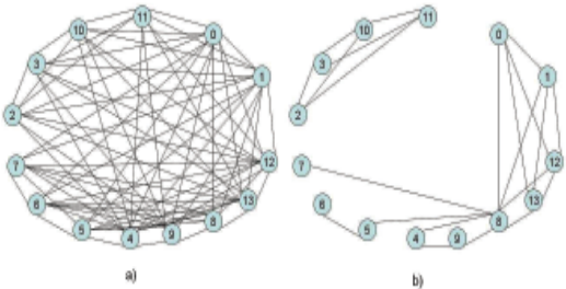
For example, Figure1 a) represents the primal graph of one of the RLFAP benchmarks. This COP P has only binary objectives, represented by the edges between nodes (variables). The second graph b) is the primal graph of P D computed by Algorithm 3 when run on P with λ = 0.4.
The induced width of P D is 3 compared to an induced width of 9 found in P. E(P D .Obj )/E(P.Obj ) = 0.76, i.e., 76% of the expected cost of the entire problem is found in the objectives of P D .
Consider the running of DB using P D . Suppose the following assignments are made: V8 ← a, V7 ← x, and V5 is selected as the next variable to assign (Line 9 of Algorithm 2). τ will be the component 〈{V5, V6}, P.Dom, {O56}〉. Kd will include components whose variables are {V0, V1, V12, V13}, {V2, V3, V10, V11}, {V4, V9} and {V6}. Note that P has not decomposed at this point in search.
5 Experiments
We have implemented the algorithms described above, and tested them on weighted-CSP (wCSP) problems with high tree-width. It should be noted that our approach is not designed for problems of low tree-width-on such problems traditional decomposition algorithms like AND-OR search and OR-Decomposition will typically be better choices.
It can also be observed that DB is able to prune the branch and bound search space either when BD ≥ GUB or BO ≥ GUB (line 5 of DB). That is, either with the bounds computed via decomposition over the subproblem P D (BD) or with the ordinary bounds computed by branch and bound (BO). Hence, there is some tension in the choice of which variable to instantiate next. Variables that encourage P D to decompose can be chosen to enable better bounds BD from P D , or variables that branch and bound would normally select (using whatever heuristic it is operating with) can be chosen to enable better bounds BO from the full problem P.
We experimented with the Earth Observing Satellites with Global Constraints (SPOT5+Global) problems. These problems involve selecting a subset of candidate photographs so that some imperative constraints are satisfied and the total importance of the selected photographs is maximized. The problems have been formulated as wCSP's with binary and ternary constraints in the SPOT5 benchmark [Bensana et al., 1999]. The original SPOT5 problems have relatively low tree-width, so to make them applicable for our experiments we have added two global constraints to every instance. 2 First we imposed a parity constraint on the assigned values, requiring that the sum of the assigned values be equal to 0 mod 2, and second we imposed a constraint requiring that the sum of the assigned values be less that 0.9 times the sum of the maximum values in the variable domains. Basic forward checking is used for both of these constraints. Since the scope of these constraints contain all of the problem's variables they make the tree-width of the problems equal to the number of variables minus one. Algorithm 3 generates a decomposible subproblem that simply excludes these two global constraints.
| Instance | BB | DB | DB+P |
|---|---|---|---|
| 1502b | 8.7 | 1.1 | 0.5 |
| 29b | 3.0 | 0.2 | 0.3 |
| 404b | 94.3 | 10.4 | 0.4 |
| 503b | - | - | 7.6 |
| 54b | 0.1 | 0.1 | 0.1 |
| 1502 | 9.4 | 1.6 | 0.6 |
| 29 | 3.2 | 0.2 | 0.4 |
| 404 | 148.3 | 158.7 | 3.1 |
| 503 | - | - | 370.9 |
| 54 | 0.4 | 0.7 | 0.3 |
Table 1 show our results on this problem suite. The SPOT5 benchmark contains 42 problems, but we only show those problems that could be solved by at least one of the tested algorithms within a 1200 second time limit when run on 2.66GHz machines with 8GB of memory. The table shows results from the following algorithms: standard branch and bound BB and our proposed decomposition bounding algorithm run with two different variable ordering heuristics, DB and DB+P. Note that standard decomposition algorithms like AND-OR search and OR-Decomposition offer no advantage over BB on these problems - the full problem never decomposes during search.
The algorithms were implemented on top of the state-ofthe art solver Toolbar [Bouveret et al., 2008], and they employ the extensive FDAC propagation method [Larrosa and Schiex, 2003] to generate strong bounds. As mentioned above, however, DB and DB+P utilize FDAC for bounding the full problem P cur and weaker forward checking to bound the subproblems D and C.
BB utilizes a standard Dom/Deg variable ordering heuristic which gives preference to variables with low current domain sizes and high degree. DB uses exactly the same Dom/Deg variable ordering. For DB+P we first compute a tree-decomposition of the subproblem D using a standard min-fill heuristic. DB+P always selects a variable from the top most unset label of this tree-decomposition, using Dom/Deg to decide which of the unset variables in this label to select first. Hence, DB+P gives priority to generating good bounds from BD by encouraging decomposition in P D , while DB gives priority to generating bounds from the full problem. All of the algorithms order the values of the selected variable using the unary objectives computed by FDAC. That is, the values for each selected variable V are branched on in order lowest unary objective cost first.
2 Note that it can often be the case that in practice when solving a COP various additional situation specific constraints have to be considered.
| Instance | NVar | IW(P) | IW(P D ) | E[PD ] E[P] |
|---|---|---|---|---|
| CELAR6-0 | 16 | 7 | 3 | 0.92 |
| CELAR6-1 | 14 | 9 | 3 | 0.77 |
| CELAR6-2 | 16 | 10 | 4 | 0.81 |
| CELAR7-2 | 16 | 10 | 4 | 0.95 |
| CELAR7-4-22 | 22 | 11 | 4 | 0.96 |
| Instance | BB | AO | OR | DB | DB+P |
|---|---|---|---|---|---|
| CELAR6-0 | 0.3 | 0.2 | 0.2 | 0.3 | 1.1 |
| CELAR6-1-24 | 9.1 | 8.6 | 10.1 | 3.6 | 3.6 |
| CELAR6-1 | 202.3 | 124.7 | 162.7 | 42.1 | 31.1 |
| CELAR6-2 | 752.6 | 373.0 | 383.0 | 73.6 | 172.2 |
| CELAR6-3 | - | 752.7 | 981.55 | 271.8 | 396.2 |
| CELAR6-4-20 | - | 22.5 | 32.42 | 26.2 | 34.9 |
| CELAR7-0 | 0.4 | 0.3 | 0.4 | 0.1 | 0.1 |
| CELAR7-1-20 | 0.2 | 0.2 | 0.2 | 0.1 | 0.2 |
| CELAR7-1 | 11.8 | 11.6 | 13.0 | 7.1 | 7.0 |
| CELAR7-2 | 239.1 | 245.4 | 248.0 | 248.9 | 206.5 |
| CELAR7-4-22 | - | 577.5 | 740.8 | 37.3 | 964.0 |
The results show that DB yields a significant improvement over BB, providing a 5 to 16 fold performance improvement on 5 of the problems, roughly the same performance on 2 of the problems, and about a 50% decrease in performance on one (very easy) problem. When the variable ordering gives preference to generating decompositions over P D however, we get a even more profound improvement, with DB+P solving two problems the other algorithms cannot solve.
Our second set of experiments are with the Radio Link Frequency Assignment Problem (RLFAP) problems. These problems involve assigning frequencies to a set of radio links so that all the links may operate together without noticeable interference. The RLFAP instances are cast as binary wCSP's [Cabon et al., 1999]. Unlike the previous experiments, we did not make any changes to these problems since many of the problems have relatively high tree-width in their original form, although we only considered problems with induced width greater than |Vars|/2.
Table 2 shows the the results of running Algorithm 3. The induced width (IW) of the original problem P and the generated decomposible subproblem P D are shown as is the proportion of expected objective cost allocated to P D . The induced widths are computed from a min-fill ordering, which only approximates the true tree width. Nevertheless, the results indicates that our heuristic approach often yields a P D that has significantly lower tree width that P, while still retaining many of the most costly objectives. The results on the other problems not shown here are quite similar.
Table 3 show our results on the RLFAP problem suite. Running with on the same machines and timeout as before the table shows the results obtained from branch and bound BB, AND-OR search AO, OR-Decomposition search OR, and our decomposition bounding algorithm DB and DB+P.
BB, DB and DB+P are as in the previous results. AO and OR first compute a tree-decomposition over the full problem using min-fill. They then operate like DB+P, selecting the Dom/Deg best variable from amongst the unset variables contained in the top most unset label of this treedecomposition. They also both use FDAC and the same value ordering scheme as the other algorithms (as described above). Finally, AO orders its components so as to solve the component with the most variables first.
The benchmark family includes 32 problems, although only 11 of the problems have high tree-width. The results shows that DB and DB+P generally perform better than the other algorithms, displaying the best performance on 9 out of the 11 problems. On this problem suite, however, there is no clear winner between DB and DB+P, indicating that on many of these problems the best bounds are generated by the original problemP. Although the results for the low-tree width instances are not reported in this paper, traditional decomposition does perform better than DB and BB. It should be noted that the tree-width of instances can be quickly estimated by, e.g., the min-fill heuristic, as a preprocessing step. If the tree-width is found to be low, traditional decomposition algorithms can be used instead of DB.
6 Conclusions
COPs can benefit greatly from decomposition, but traditional decomposition techniques are ineffective on problems with high tree-width. In this paper, we have introduced a way of exploiting decomposition on such problems that is compatible with a fully flexible branch and bound search employing dynamic variable and value ordering. We have tested this method on a number of benchmarks, and showed that it can yield improvements over current state-of-the-art algorithms.
@inproceedings{ijcai2009p94,
  title     = {Exploiting Decomposition on Constraint Problems with High Tree-Width},
  author    = {Kitching, Matthew and Bacchus, Fahiem},
  booktitle = {Proceedings of the Twenty-First International Joint Conference on
               Artificial Intelligence, {IJCAI-09}},
  publisher = {International Joint Conferences on Artificial Intelligence},
  editor    = {Craig Boutilier},
  pages     = {525--530},
  year      = {2009},
  url       = {https://ijcai.org/proceedings/2009/94},
}
TY - CPAPER TI - Exploiting Decomposition on Constraint Problems with High Tree-Width AU - Kitching, Matthew AU - Bacchus, Fahiem T2 - Proceedings of the Twenty-First International Joint Conference on Artificial Intelligence, IJCAI-09 PB - International Joint Conferences on Artificial Intelligence PY - 2009 SP - 525 EP - 530 UR - https://ijcai.org/proceedings/2009/94 ER -Copied
Machine-readable versions of this paper, for tools and AI agents:





