
AND/OR Branch-and-Bound for Graphical Models
Proceedings of the Nineteenth International Joint Conference on Artificial Intelligence. Pages 224-228.
© 2005 International Joint Conferences on Artificial Intelligence
Abstract
The paper presents and evaluates the power of a new framework for optimization in graphical models, based on AND/OR search spaces. The virtue of the AND/OR representation of the search space is that its size may be far smaller than that of a traditional OR representation. We develop our work on Constraint Optimization Problems (COP) and introduce a new generation of depth-first Branch-and-Bound algorithms that explore an AND/OR search space and use static and dynamic mini-bucket heuristics to guide the search. We focus on two optimization problems, solving Weighted CSPs (WCSP) and finding the Most Probable Explanation (MPE) in belief networks. We show that the new AND/OR approach improves considerably over the classic OR space, on a variety of benchmarks including random and real-world problems. We also demonstrate the impact of different lower bounding heuristics on Branch-and-Bound exploring AND/OR spaces.
- [Bayardo and Miranker, 1995] R. Bayardo and D. Miranker. On the space-time trade-off in solving constraint satisfac- tion problems. Proc. of IJCAI'95, 1995. IJCAI
- [Bistarelli et al., 1997] S. Bistarelli, U. Montanari, and F. Rossi. Semiring based constraint solving and optimiza- tion. Journal of ACM, 44(2):309-315, 1997.
- [Cabon et al., 1999] B. Cabon, S. de Givry, L. Lobjois, T. Schiex, and J. Warners. Radio link frequency assign- ment. Constraints, (4):79-89, 1999.
- [Dechter and Mateescu, 2004] R. Dechter and R. Mateescu. Mixtures of deterministic-probabilistic networks. Proc. of UAI'04, 2004.
- [Dechter and Rish, 2003] R. Dechter and I. Rish. Mini- buckets: A general scheme for approximating inference. Journal of ACM, 2003.
- [Dechter, 1999] R. Dechter. Bucket elimination: A unifying framework for reasoning. Artificial Intelligence, 113:41- 85, 1999.
- [Freuder and Quinn, 1985] E. Freuder and M. Quinn. Taking advantage of stable sets of variables in constraint satisfac- tion problems. Proc. of IJCAI'85, 1985. IJCAI
- [Jegou and Terrioux, 2004] P. Jegou and C. Terrioux. Decom- position and good recording for solving max-csps. Proc. of ECAI'04, 2004.
- [Kanal and Kumar, 1988] L. Kanal and V. Kumar. Search in artificial intelligence. Springer-Verlag., 1988.
- [Kask and Dechter, 2001] K. Kask and R. Dechter. A general scheme for automatic generation of search heuristics from specification dependencies. Artificial Intelligence, 2001.
- [Larrosa and Schiex, 2003] J. Larrosa and T. Schiex. In the quest of the best form of local consistency for weighted csp. Proc. of IJCAI'03, pages 631-637, 2003. IJCAI
- [Larrosa et al., 2002] J. Larrosa, P. Meseguer, and M. Sanchez. Pseudo-tree search with soft constraints. Proc. of ECAI'02, 2002.
- [Meseguer et al., 1999] P. Meseguer, J. Larrosa, and T. Schiex. Maintaining reversible dac for max-csp. Artificial Intelligence, 107(1):149-163, 1999.
- [Pearl, 1988] J. Pearl. Probabilistic Reasoning in Intelligent Systems. Morgan-Kaufmann, 1988.
References were extracted automatically from the PDF and may contain errors.
Full text extracted automatically from the PDF; figures, tables and equations may differ. The PDF is the version of record.
1 Introduction
Graphical models such as constraint networks and belief networks have become a powerful representation framework for reasoning with deterministic and probabilistic information. These models use graphs to capture conditional independencies between variables, allowing a concise representation of the knowledge as well as efficient graph-based query processing algorithms.
Optimization tasks such as finding the most likely state of a belief network or finding a solution that violates the least number of constraints in a constraint network are all instances of Constraint Optimization Problems (COP). They are typically tackled with either search or inference algorithms. Search methods (e.g. depth-first Branch-and-Bound, best-first search) are time exponential in the number of variables and can operate in polynomial space. Inference algorithms (e.g. variable elimination, tree-clustering) are time and space exponential in a topological parameter called tree width. If the tree width is large, the high space complexity makes the latter methods impractical.
In this paper we focus on search. In contrast to inference algorithms, search algorithms are less sensitive to the graph-model structure because they traverse a structureblind search space. To overcome this problem the idea of AND/OR search spaces was introduced in the past year, and was shown to vividly display independencies encoded in the underlying graphical model [Dechter andMateescu, 2004]. In this paper we develop AND/OR Branch-and-Bound (AOBB), a general algorithm for solving COPs, which explores the AND/OR search tree in a depth-first manner. Its efficiency depends on its guiding heuristic functions. In the past, a class of partitioning-based heuristic functions, based on the Mini-Bucket approximation and known as static mini-bucket heuristics was shown to be powerful for optimization problems [Kask and Dechter, 2001]. We take the idea one step further and introduce dynamic mini-bucket heuristics, which are computed dynamically at each node of the search tree. Both schemes are parameterized by the Mini-Bucket i-bound, which allows for a controllable trade-off between preprocessing and search.
We apply the AND/OR algorithms to two common optimization problems: solving Weighted CSPs [Bistarelli et al., 1997] and finding the Most Probable Explanation (MPE) in belief networks [Pearl, 1988]. We experiment with both random models and real-world benchmarks. Our results show conclusively that the new AND/OR Branch-and-Bound algorithms improve dramatically over traditional OR ones, especially when the heuristic estimates are inaccurate and the algorithms rely primarily on search rather than on pruning.
2 Background
A finite Constraint Optimization Problem (COP) is a six-tuple P = 〈X,D,F,⊗, ⇓,Z〉, where X = {X1, ...,Xn} is a set of variables, D = {D1, ...,Dn} is a set of finite domains and F = {f1, ..., fm} is a set of constraints. Constraints can be either soft (cost functions) or hard (sets of allowed tuples). Without loss of generality we assume that hard constraints are represented as (bi-valued) cost functions. Allowed and forbidden tuples have cost 0 and ∞, respectively. The scope of function fi, denoted scope(fi) ⊆ X, is the set of arguments of fi. The operators ⊗ and ⇓ can be defined using the semi-ring framework [Bistarelli et al., 1997], but in this paper we assume that: ⊗ifi is a combination operator, ⊗ifi ∈ {∏i fi, ∑i fi} and ⇓Y f is an elimination operator, ⇓Y f ∈ {maxS-Y f,minS-Y f}, where S is the scope of function f and Y ⊆ X. The scope of ⇓Y f is Y .
An optimization task is defined by g(Z) = ⇓Z⊗mi=1 fi, where Z ⊆ X. A global optimization is the task of finding the best global cost, namely Z = ∅. For simplicity we will develop our work assuming a COP instance with summation and minimization as combination and elimination operators, and a global cost function defined by f(X) = minX ∑mi=1 fi.
The primal graph of a COP instance has the variables X as its nodes and an arc connects any two variables that appear in the scope of the same function.
In practice, most complete COP solvers follow a depth-first Branch-and-Bound strategy which maintains an upper bound, the best solution cost found so-far, and a lower bound on the optimal extension of the current assignment. Value pruning occurs as soon as the lower bound exceeds the upper bound.
3 AND/OR Search Spaces
The usual way to do search (i.e. OR search) is to instantiate variables in turn, following a static/dynamic linear ordering. This process defines a search tree (i.e. OR tree), whose nodes represent states in the space of partial assignments.
One way to exploit the independencies encoded by the graphical model is to introduce AND nodes into the search space, which will decompose the problem into separate subproblems. In the past year, [Dechter and Mateescu, 2004] introduced the concept of AND/OR search spaces for constraint networks, belief networks, and for graphical models in general. The AND/OR search space is defined using a back-bone pseudo-tree arrangement of the primal graph.
DEFINITION 1 (pseudo-tree) Given the primal graph G of a COP instance P, a pseudo-tree is a rooted tree with the same set of vertices as G and has the property that adjacent vertices from G must be in the same branch of the rooted tree [Freuder and Quinn, 1985].
DEFINITION 2 (AND/OR search tree) Given a COP instance P, its primal graph G and a pseudo-tree T of G, the associated AND/OR search tree ST (P) has alternating levels of OR nodes and AND nodes. The OR nodes are labeled Xi and correspond to the variables. The AND nodes are labeled 〈Xi, a〉 and correspond to value assignments in the domains of the variables. The root of the AND/OR search tree is an OR node, labeled with the root of T . The children of an OR node Xi are AND nodes labeled with assignments 〈Xi, a〉, consistent along the path from the root. The children of an AND node 〈Xi, a〉 are OR nodes labeled with the children of variable Xi in T . The path of a node n ∈ ST , denoted PathST (n), is the path from the the root of ST to n, and corresponds to a partial value assignment to all variables along the path.
A solution subtree SolST of ST is an AND/OR subtree such that:(i) it contains the root of ST ;(ii) if a nonterminal AND node n ∈ ST is in SolST then all of its children are in SolST ;(iii) if a nonterminal OR node n ∈ ST is in SolST then exactly one of its children is in SolST .
Example 1 Consider the graphical model in Figure 1(a) (top) describing a graph coloring problem over domains {0,1}. An AND/OR search tree based on the pseudo-tree in Figure 1(a) (bottom), and a highlighted solution subtree are given in Figure 1(b). Observe that the AND node 〈B, 0〉1 roots two independent subproblems, one represented by variable {E}, and the other by variables {C, D, F}.
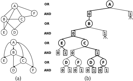
THEOREM 1 ([Dechter and Mateescu, 2004]) Given a COP instance P and a pseudo-tree T , its AND/OR search tree ST is sound and complete (contains all and only solutions) and its size is O(n·exp(m)), where m is the depth of the pseudo-tree.
Any search algorithm that traverses the AND/OR search tree in a depth-first manner is guaranteed to have a time complexity exponential in the depth of the pseudo-tree and can operate in linear space. In contrast, the time complexity of search algorithms exploring traditional OR search trees is exponential in the number of variables. The arcs in ST are annotated by appropriate labels of the cost functions. The nodes in ST can be associated with a value, accumulating the result of the computation resulted from the subtree below.
DEFINITION 3 (label) The label l(Xi, 〈Xi, a〉) of the arc from the OR node Xi to the AND node 〈Xi, a〉 is defined as the sum of all the cost functions values for which variable Xi is contained in their scope and whose scope is fully assigned along P athST (〈Xi, a〉).
DEFINITION 4 (value) The value v(n) of a node n ∈ ST , is defined recursively as follows: (i) if n = 〈Xi, a〉 is a terminal AND node then v(n) = l(Xi, 〈Xi, a〉); (ii) if n = 〈Xi, a〉 is an internal AND node then v(n) = l(Xi, 〈Xi, a〉)+ ∑n′∈succ(n) v(n′ ); (iii) if n = Xi is an internal OR node then v(n) = minn′∈succ(n)v(n′ ), where succ(n) are the children of n in ST .
Clearly, the value of each node can be computed recursively, from leaves to root. We can show that:
PROPOSITION 1 Given an AND/OR search tree ST of a COP instance P = 〈X,D,F,+,min〉, the value function v(n) is the minimal cost solution to the subproblem rooted at n, subject to the current variable instantiation along the path from root to n. If n is the root of ST , then v(n) is the minimal cost solution to P.
Therefore, we can traverse the AND/OR search tree in a depth-first manner to compute the value of the root. This approach would require linear space, storing only the current partial solution subtree. The algorithm expands alternating levels of OR and AND nodes, periodically evaluating the value function of the nodes along the current path. It terminates when the root node is evaluated with the optimal cost.
1 In the figure we only denote the value. 〈B, 0〉 is written as 0 child of B.
4 AND/ORBranch and Bound
If each node n at the search frontier is assigned a heuristic lower-bound estimate h(n) of v(n), then we can calculate the most promising extension of the current partial solution subtree and prune the portion of the search space that becomes irrelevant, as part of a Branch-and-Bound scheme. We call h(n) a static heuristic function.
4.1 Lower Bounds on Partial Solution Trees
At any stage of the search, the current partial solution is a partial solution subtree, denoted PST . By the nature of the search process, PST must be connected, must contain the root node and will have a frontier containing all those nodes that were generated but not yet expanded. The leaves of PST are called tip nodes. In this section we will define a dynamic heuristic function of a node n relative to the current PST , which yields a more accurate lower bound on v(n) than h(n). For that we introduce the notions of active path, its inside and outside contexts and the active partial subtree.
DEFINITION 5 Given the current PST , the active path AP(t) is the path of assignments from the root of PST to the current tip node t. The inside context in(AP) of AP(t) contains all nodes that were fully evaluated and are children of nodes on AP(t). The outside context out(AP) of AP(t), contains all nodes that were generated but not yet expanded and are children of the nodes on AP(t). The active partial subtree APT (n) rooted at a node n ∈ AP(t) contains the sub-path between n and t, and all OR children of the AND nodes on it.
For illustration consider the partial solution subtree in Figure 2(b) based on the pseudo-tree in Figure 2(a). The active path AP(t) has tip node t = 〈E, 1〉, namely it is (A = 1, B = 1,E = 1). The shaded nodes at the left of AP(t) are in in(AP) and their corresponding subtrees have already been explored. out(AP) includes the nodes {C, F}, which are also in the search frontier. The active partial subtree APT (B) is highlighted. It contains the nodes {B, 〈B, 1〉,E, 〈E, 1〉} on AP(t), the OR node D from in(AP) and the OR node F from out(AP).
DEFINITION 6 (dynamic lower bound) Given an active partial tree APT (n), the dynamic heuristic evaluation function of n, fh(n), is defined recursively as follows: (i) if APT (n) consists only of a single node n, and if n ∈ in(AP) then fh(n) = v(n) else fh(n) = h(n); (ii) if n = 〈Xi, a〉 is an AND node, having OR children m1, ...,mk then fh(n) = max(h(n), l(Xi, 〈Xi, a〉) + ∑ki=1 fh(mi)); (iii) if n = Xi is an OR node, having an AND child m, then fh(n) = max(h(n), fh(m)).
We can prove that fh(n) is a lower bound on the optimal solution cost to the subproblem rooted at n, namely fh(n) ≤ v(n), and also by definition fh(n) ≥ h(n), indicating that the dynamic lower bound is superior to the static one.
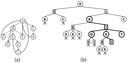
Example 2 For the active partial subtree rooted at B in Figure 2(b), the lower bound fh(B) on v(B) is computed recursively as follows: fh(B) = max(h(B), fh(〈B, 1〉)), where fh(〈B, 1〉) = max(h(〈B, 1〉), l(B, 〈B, 1〉)+v(D)+fh(E)+ h(F)). Similarly, fh(E) = max(h(E), fh(〈E, 1〉)) = max(h(E), h(〈E, 1〉)), since fh(〈E, 1〉) = h(〈E, 1〉).
4.2 The Branch-and-Bound Procedure
In the AND/OR search space, we can calculate a lower bound on v(n) of a node n on the active path, by using fh(n). In addition, we can compute an upper bound on v(n), based on the portion of the search space below n that has already been explored. The upper bound ub(n) on v(n) is the current minimum cost solution subtree of the subproblem rooted at n.
In Figure 2(b), the upper bound on v(B) is ub(B) = min(∞, v(〈B, 0〉)) = v(〈B, 0〉), and it represents the current best cost solution rooted at B. The lower bound fh(B) on v(B) is calculated as seen in the previous example. If fh(B) ≥ ub(B), then searching below t = 〈E, 1〉 of the active path is guaranteed not to reduce ub(B) and therefore, the subtree rooted at 〈E, 1〉 can be pruned.
PROPOSITION 2 (pruning rule) Given the active path AP(t) of a current PST , for any node n on AP(t), if fh(n) ≥ ub(n) then pruning the subtree below t is safe.
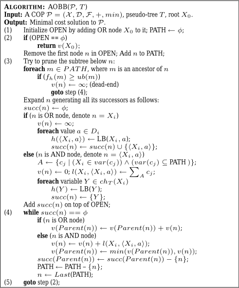
A depth-first AND/OR Branch-and-Bound (AOBB) algorithm that implements this pruning rule is described in Figure 3. A list called OPEN simulates the recursion stack. The list PATH maintains the current assignment (i.e. the active path). Parent(n) refers to the predecessor of n in PATH, which is also the parent in the AND/OR tree, succ denotes the set of successors of a node in the AND/OR tree and chT (Xi) denotes the children of variable Xi in T . Procedure LB(n) computes the static heuristic estimate h(n) of v(n).
Step (3) is where the search goes forward and expands alternating levels of OR and AND nodes. Upon the expansion of n, the algorithm successively updates the lower bound function fh(m) for every ancestor m of n along the active path, and discontinues search below n if, for some m, fh(m) ≥ ub(m).
Step (4) is where the value functions are propagated backward. This is triggered when a node has an empty set of successors and it typically happens when the node's descendants are all evaluated or when it is a dead-end. Clearly,
THEOREM 2 AOBB is sound and complete for COP.
While the time complexity of algorithm AOBB is bounded by O(n · exp(m)), the size of the AND/OR search space, the pruning rule is designed to yield a far better complexity.
5 Specific Lower Bound Heuristics
In this section we describe briefly two general schemes for generating static heuristic estimates h(n), based on the MiniBucket approximation. These schemes are parameterized by the Mini-Bucket i-bound, thus allowing for a controllable trade-off between heuristic strength and its overhead. We also mention a third scheme which is based on the notion of directional arc-consistency and is specific to the WCSP model.
5.1 TheMini-Bucket Heuristics
Mini-Bucket Elimination (MBE) [Dechter and Rish, 2003] is an approximation algorithm designed to avoid the high time and space complexity of Bucket Elimination (BE) [Dechter, 1999], by partitioning large buckets into smaller subsets, called mini buckets, each containing at most i (called i-bound) distinct variables. The mini-buckets are then processed separately. The algorithm outputs not only a bound on the optimal solution cost, but also the collection of augmented buckets, which form the basis for the heuristics generated. The complexity is time and space O(exp(i)).
Static Mini-Bucket Heuristics In the past, [Kask and Dechter, 2001] showed that the intermediate functions generated by the Mini-Bucket algorithm MBE(i) can be used to compute a heuristic function, that underestimates the minimal extension of the current assignment in a regular OR search tree. In this paper we extend the idea to AND/OR search spaces as well. For that, assume that a COP instance P with pseudo-tree T is being solved by AOBB search, where the active path ends with some OR node Xj. Consider also the augmented bucket structure {B(X1), ...,B(Xn)} of P, constructed along the ordering resulted from a DFS traversal of T . For each possible value assignment Xj = xj , the static minibucket heuristic estimate h(xj) of the minimal cost solution rooted at Xj can be computed as the sum of the original functions in bucket B(Xj) and the intermediate functions λk that were generated in buckets B(Xk), where Xk is a descendant of Xj in T (more details in [Kask and Dechter, 2001]).
Dynamic Mini-Bucket Heuristics This idea can be pushed one step further. Rather than pre-compiling the mini-bucket heuristic information, it is possible to generate it dynamically, during search. Therefore, the dynamic mini-bucket heuristic computes a lower bound by the Mini-Bucket algorithm MBE(i), at each node n in the search space, restricted to the subproblem rooted at n and subject to the current partial instantiation. Specifically, h(xj) is calculated as the sum of the original and λk functions residing in bucket B(Xj), where λk 's are computed in buckets B(Xk) of Xj's descendants in T , conditioned on the current assignment of the active path.
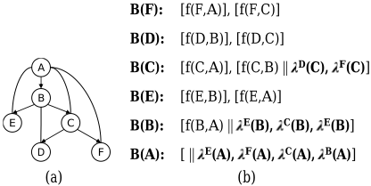
Example 3 Figure 4(b) shows the augmented bucket structure generated by MBE(i=2) for the binary COP instance displayed in Figure 4(a), along the ordering (A, B, E, C, D, F ); square brackets denote the choice of partitioning. Assume that during search, the active path of the current partial solution subtree is (A = a,B = b) and the tip node is the OR node C. The static mini-bucket heuristic estimate h(C = c) = f (c, a) + f (c, b) + λF (a) + λF (c) + λD (c) + λD (b). The dynamic mini-bucket heuristic estimate h(C = c), involves the same λ functions generated in buckets B(F) and B(D), only that the λ's are now computed dynamically, conditioned on the current partial assignment (A = a, B = b).
5.2 Directional Arc-Consistency Heuristics
We also adapted for the AND/OR search space two other successful heuristics generators, reversible DAC counts (RDAC) [Meseguer et al., 1999] and maintaining full DAC (MFDAC) [Larrosa and Schiex, 2003], which proved powerful for solving binary Weighted CSPs (details omitted for space reasons).
6 Experiments
In this section we evaluate empirically the performance of our new AND/OR Branch-and-Bound approach on two classes of optimization problems: Weighted CSP (WCSP) and the Most Probable Explanation (MPE) problem in belief networks 2 .
| Network (n,d,c,t) [w*,h] connectivity | s-AOMB s-BBMB d-AOMB d-BBMB i=2 | s-AOMB s-BBMB d-AOMB d-BBMB i=4 | s-AOMB s-BBMB d-AOMB d-BBMB i=6 | s-AOMB s-BBMB d-AOMB d-BBMB i=8 | AORDAC BBRDAC AOMFDAC BBMFDAC | |||||
|---|---|---|---|---|---|---|---|---|---|---|
| time | nodes | time | nodes | time | nodes | time | nodes | time | nodes | |
| (20,5,100,0.7) [12,15] medium | - - 74.43 124.45 | 2.4M 6.3M 90K 523K | 115.57 179.34 51.19 80.79 | 2.5M 7.6M 6.9K 34K | 15.49 127.77 104.08 140.10 | 408K 6.5M 751 3.3K | 6.91 45.76 169.30 176.33 | 126K 2.2M 101 537 | 21.70 24.74 9.99 8.75 | 441K 1.3M 20K 21.3K |
| (30,5,90,0.7) [11,16] low | - - | 2.8M 6M 82K | 105.77 180.00 | 2.2M 7.5M 4.3K | 9.84 68.90 63.07 | 262K 3.3M 548 | 2.71 5.64 94.95 | 28K 230K 111 | 78.50 78.24 10.72 | 1.3M 4.2M 22.2K |
| 72.94 | 348K | 31.85 | 22K | 90.70 | 123.42 | 265 | 8.79 | 31.4K | ||
| (50,5,80,0.7) [8,16] sparse | 104.15 67.53 | 1.4M | 69.49 1.80 | 57K | 0.12 | 1.7K 2.6K | ||||
| 0.62 | 28.90 | |||||||||
| - | 5M | 145.39 | 24.47 | 804K | 1.58 | 36K | ||||
| 7.91 | 4.3M | 356 | 155.58 | 691K 3.9M | ||||||
| 87 | 8.5K | |||||||||
| 63.50 | 18.6K 295K | 1.17 1.83 | 430 1K | 0.95 0.94 | 112 | 2.31 2.34 | 60 69 | 1.48 1.49 | 14K | |
Weighted CSP [Bistarelli et al., 1997; Larrosa and Schiex, 2003] extends the classic CSP formalism with so-called soft constraints which assign positive integer costs to forbidden tuples (allowed tuples have cost 0). The goal is to find a complete assignment with minimum aggregated cost. The model has numerous applications in domains such as resource allocation, combinatorial auctions or bioinformatics.
Belief Networks [Pearl, 1988] provide a formalism for reasoning under conditions of uncertainty. A belief network represents a joint probability distribution over the variables of interest. A function of the graphical model encodes conditional probability distribution of a variable given its parents in the graph (also viewed as a cost function were each tuple has associated a real cost between 0 and 1). The MPE problem is the task of finding a complete assignment with maximum probability that is consistent with the evidence. It appears in applications such as speech recognition or medical diagnosis.
The pseudo-tree was created as suggested in [Bayardo and Miranker, 1995], by a DFS traversal of the induced graph. The latter was computed using the min-fill heuristic. All competing algorithms were restricted to a static variable ordering resulted from a DFS traversal of the pseudo-tree. We report the average effort, as CPU time (in seconds) and number of visited nodes (AND nodes only for the AND/OR algorithms), required for proving optimality of the solution. For all test instances we record the number of variables (n), domain size (d), number of functions (c), induced width (w*) and height of the pseudotree (h). A "-" indicates that a time limit was exceeded by the respective algorithm. The best results are highlighted.
6.1 Weighted CSP
For this domain we experimented with random binary WCSP problems as well as real-world benchmarks. We consider four classes of AND/OR Branch-and-Bound (AOBB) algorithms, each using a specific heuristics generator, as follows. Classes s-AOMB/d-AOMB are guided by static/dynamic mini-bucket heuristics, AORDAC uses RDAC based heuristics, and AOMFDAC maintains full DAC. For comparison, we include results obtained with the classic OR version of each class of algorithms, denoted here by s-BBMB, d-BBMB, BBRDAC and BBMFDAC, respectively.
2 All our experiments were done on a 2.4GHz Pentium IV with 1GB of RAM, running Windows XP
| Network | (n,d,c,w*,h) | BBMFDAC | AOMFDAC | ||
|---|---|---|---|---|---|
| time (sec) | nodes | time (sec) | nodes | ||
| CELAR6-SUB0 | (16,44,57,7,10) | 2.78 | 1,871 | 1.98 | 435 |
| CELAR6-SUB1 | (14,44,75,9,11) | 2420.93 | 364,986 | 981.98 | 180,784 |
| CELAR6-SUB2 | (16,44,89,10,13) | 8801.12 | 19,544,182 | 1138.87 | 175,377 |
| CELAR6-SUB3 | (18,44,106,10,13) | 38889.20 | 91,168,896 | 4028.59 | 846,986 |
| CELAR6-SUB4 | (22,44,131,11,16) | 84478.40 | 6,955,039 | 47115.40 | 4,643,229 |
Random Binary Networks
Our random binary WCSP class is characterized by a five parameter model 〈n, d, c, t,w〉 [Larrosa and Schiex, 2003], where n is the number of variables, d the domain size, c the number of constraints, and t the constraint tightness defined as the ratio of forbidden tuples. The costs of inconsistent tuples are uniformly randomly distributed between 1 and w.
Table 1 shows results for experiments with three problem classes containing instances with medium, low and very low connectivity. We chose a maximum penalty cost w of 10 and set the constraint tightness to 70% in order to obtain overconstrained problems. For each problem class we generated 20 instances and the time limit was set to 180 seconds. The columns are indexed by the i-bound of the mini-bucket heuristics. When comparing AND/OR versus OR algorithms we notice a considerable improvement in terms of CPU time and number of nodes visited, especially for problems with low and very low connectivity. This observation verifies the theory because a relatively sparse problem is likely to produce a shallow pseudo-tree, which in turn enhances the performance of the AND/OR algorithms. In terms of the quality of the heuristics, we also observe that the static mini-buckets with a relatively large i-bound represent the best choice. However, if large i-bounds are not possible, dynamic mini-buckets with small i-bounds are preferred, especially for sparse problems. For medium and low connected problems, MFDAC proves to be cost effective with respect to the other heuristics generators.
Radio Link Frequency Assignment Problem (RLFAP)
RLFAP is a communication problem where the goal is to assign frequencies to a set of radio links in such a way that all links may operate together without noticeable interferences [Cabon et al., 1999]. It can be naturally casted as a binary WCSP where each forbidden tuple has an associated penalty cost. Table 2 compares algorithms BBMFDAC and AOMFDAC for solving 5 publicly available RLFAP subinstances called CELAR6-SUBi (i = 0, ..., 4). We can see that the AND/OR approach is beneficial for this domain as well. In CELAR6-SUB4, the hardest instance, AOMFDAC causes a CPU speed up of 1.8, whereas in CELAR6-SUB3 the speed up is as much as 9.6. We also compared AOMFDAC against BTD, a recent algorithm introduced in [Jegou and Terrioux, 2004]. BTD solves the MAX-CSP version of CELAR6-SUB4 (i.e. 0/1 penalty costs) in about 123,000 sec., whereas AOMFDAC proves optimality in only 2,574 sec. The performance of the mini-bucket based algorithms was quite poor on this domain, due to the very low quality of the heuristic estimates resulted from approximating subproblems with very large domains (up to 44 values).
| Network (n,d,w*,h) | s-AOMB s-BBMB d-AOMB d-BBMB i=2 | s-AOMB s-BBMB d-AOMB d-BBMB | s-AOMB s-BBMB d-AOMB d-BBMB i=4 | s-AOMB s-BBMB d-AOMB d-BBMB i=5 | ||||
|---|---|---|---|---|---|---|---|---|
| time | nodes | i=3 time | nodes | time | nodes | time | nodes | |
| Mildew (35,100,4,15) | 4.58 - 86.38 162.61 | 55K 26M 15K | 0.50 233.86 34.45 41.92 | 5,465 6.9M 1,424 | 0.28 0.47 1.69 | 35 4,970 35 363 | 0.66 0.81 3.02 3.13 | 35 4,940 35 363 |
| Barley (48,67,7,17) | - - - | 83K 8.5M 16M 79K | - - 135.97 | 5,113 7.6M 18M 23K | 1.78 46.22 - 12.55 | 807K 17M 667 | 0.56 - 45.95 | 9.6K 14M 567 |
| Munin1 (189,21,11,24) | - 57.36 - 66.56 | 2.2M 1.2M 8.5M 185K 405K | - 12.08 - 12.47 | 1K 260K 9.2M 8.1K | 346.08 7.20 - 10.30 | 76K 172K 9.9M 1.6K | - 1.66 - 11.99 | 86K 43K 523 |
| Munin2 | - | - | 430K | - | 235K | 14.63 | 8.3K 917 | |
| (1003,21,7,35) | - - - | 5.6M 1.7M 3.2M | - - - | 6.7M 2.7M 1.2M | 116.19 - 524.54 - | 1.8M 430K 299K | 1.64 - | 21K 428K 3.8K |
| Munin3 (1044,21,7,25) | - - - | 33K 5.9M | - - - | 131K 4.9M | 1.31 - | 101K 17K | 39.22 - | 20K 6.2K |
| Pigs (441,3,10,27) | - - | 1.4M 2.4M 33K | 1.2M 58K | 3.59 - | 316K 5.9K | 0.45 - 2.84 | 1.5M 3.8K | |
| 68.64 | 31K | |||||||
| - | 15M | - | 125K | 0.02 | 52K 441 | - 0.02 | 441 | |
| - | 2.8M | 441 | 0.63 | 4K | 0.61 | 4K | ||
| 4.2K | ||||||||
| 0.63 | ||||||||
| 0.02 | ||||||||
| - | 6.5M 2.2M | 0.08 1.03 | 441 | 0.08 | 441 | 0.11 | 441 | |
| 614 | 1.08 | 614 | 614 | |||||
| 1.11 | ||||||||
6.2 Belief Networks
For the MPE domain we also experimented with random networks and real-world benchmarks, but we only report on the latter due to space limitations. We compare the algorithms using the mini-bucket based heuristics generators, namely sAOMB, d-AOMB, s-BBMB and d-BBMB. Notice that sBBMB is currently one of the best performing complete algorithms for this domain [Kask and Dechter, 2001]
Table 3 summarizes the results for experiments on 6 realworld belief networks from the Bayesian Network Repository 3 . The time limit was set to 600 seconds. We observe again a considerable improvement of the new AND/OR algorithms over the corresponding OR ones. If we look, for example, at the Mildew instance, s-AOMB(3) causes a CPU speedup of 468 over s-BBMB(3). In conclusion, d-AOMB is superior for relatively small i-bounds (e.g. Barley, Munin3), whereas s-AOMB dominates for larger i-bounds.
7 Conclusion
The paper investigates the impact of the AND/OR search space for graphical models on optimization tasks. We introduce a general AND/OR Branch-and-Bound algorithm and specialize it with several schemes for generating heuristic estimates that can guide the search. We focus on two common optimization problems, WCSP and Bayesian MPE, and show empirically that the new AND/OR algorithms improve dramatically over traditional OR ones on a variety of benchmarks including random and real-world problems.
Our approach leaves room for future improvements. For instance, it can be modified to traverse an AND/OR graph, rather than a tree, via caching. We should consider the effect of dynamic variable ordering. Also, we used a rather simple scheme of generating pseudo-tree arrangements, probably having non-optimal height.
3 http://www.cs.huji.ac.il/labs/compbio/Repository
Related Work: AOBB is related to the Branch-and-Bound method proposed by [Kanal and Kumar, 1988] for acyclic AND/OR graphs and game trees. More recently, [Larrosa et al., 2002] extended pseudo-tree search [Freuder and Quinn, 1985] to optimization tasks in order to boost the Russian Doll search for solving Weighted CSPs. The optimization method developed in [Jegou and Terrioux, 2004] can also be interpreted as an AND/OR search graph algorithm, however it is not a linear space algorithm.
Acknowledgments
This work was supported in part by the NSF grant IIS0412854 and the MURI ONR award N00014-00-1-0617.
@inproceedings{ijcai2005p206,
  title     = {AND/OR Branch-and-Bound for Graphical Models},
  author    = {Marinescu, Radu and Dechter, Rina},
  booktitle = {Proceedings of the Nineteenth International Joint Conference on
               Artificial Intelligence, {IJCAI-05}},
  publisher = {International Joint Conferences on Artificial Intelligence},
  editor    = {Leslie Pack Kaelbling and Alessandro Saffiotti},
  pages     = {224--228},
  year      = {2005},
  url       = {https://ijcai.org/proceedings/2005/206},
}
TY - CPAPER TI - AND/OR Branch-and-Bound for Graphical Models AU - Marinescu, Radu AU - Dechter, Rina T2 - Proceedings of the Nineteenth International Joint Conference on Artificial Intelligence, IJCAI-05 PB - International Joint Conferences on Artificial Intelligence PY - 2005 SP - 224 EP - 228 UR - https://ijcai.org/proceedings/2005/206 ER -Copied
Machine-readable versions of this paper, for tools and AI agents:





