
Stratified Planning
Proceedings of the Twenty-First International Joint Conference on Artificial Intelligence. Pages 1665-1669.
© 2009 International Joint Conferences on Artificial Intelligence
Abstract
Most planning problems have strong structures. They can be decomposed into subdomains with causal dependencies. The idea of exploiting the domain decomposition has motivated previous work such as hierarchical planning and factored planing. However, these algorithms require extensive backtracking and lead to few efficient general-purpose planners. On the other hand, heuristic search has been a successful approach to automated planning. The domain decomposition of planning problems, unfortunately, is not directly and fully exploited by heuristic search. We propose a novel and general framework to exploit domain decomposition. Based on a structure analysis on the SAS+ planning formalism, we stratify the sub-domains of a planning problem into dependency layers. By recognizing the stratification of a planning structure, we propose a space reduction method that expands only a subset of executable actions at each state. This reduction method can be combined with state-space search, allowing us to simultaneously employ the strength of domain decomposition and high-quality heuristics. We prove that the reduction preserves completeness and optimality of search and experimentally verify its effectiveness in space reduction.Yixin Chen, You Xu, Guohui Yao
- [Amir and Engelhardt, 2003] E. Amir and B. Engelhardt. Factored planning. In Proc. IJCAI, 2003.
- [Bäckström and Nebel, 1995] C. Bäckström and B. Nebel. Complexity results for SAS+ planning. Computational In- telligence, 11:17-29, 1995. IJCAI
- [Brafman and Domshlak, 2006] R. Brafman and C. Domsh- lak. Factored planning: How, when, and when not. In Proc. AAAI, 2006.
- [Helmert and Röger, 2008] M. Helmert and G. Röger. How good is almost perfect. In Proc. AAAI, 2008.
- [Helmert, 2006] M. Helmert. The Fast Downward plan- ning system. Journal of Artificial Intelligence Research, 26:191-246, 2006.
- [Kelareva et al., 2007] E. Kelareva, O. Buffet, J. Huang, and S. Thiébaux. Factored planning using decomposition trees. In Proc. IJCAI, 2007. IJCAI
- [Knoblock, 1994] C. Knoblock. Automatically generating abstractions for planning. Artificial Intelligence, 68:243- 302, 1994.
- [Lansky and Getoor, 1995] A. Lansky and L. Getoor. Scope and abstraction: two criteria for localized planning. In Proc. AAAI, 1995. IJCAI
References were extracted automatically from the PDF and may contain errors.
Full text extracted automatically from the PDF; figures, tables and equations may differ. The PDF is the version of record.
1 Introduction
We have witnessed significant improvement of the capability of automated planners in the past decade. Heuristic search remains one of the key, general-purpose approaches to planning. The performance improvement is largely due to the development of high-quality heuristics. However, as shown by recent work, developing better heuristics only has some fundamental limitations [Helmert and R¨oger, 2008]. Heuristic planners still face scalability challenges for large-scale problems. It is important to develop new, orthogonal ways to improve the efficiency, among which domain decomposition has been an attractive idea to planning researchers.
A representative work based on domain decomposition is the automated hierarchical planning methods [Knoblock,
1994; Lansky and Getoor, 1995] that utilize hierarchical factoring of planning domains. However, they typically do not scale well since they require extensive backtracking across subdomains. Another work is the factored planning approach [Amir and Engelhardt, 2003; Brafman and Domshlak, 2006; Kelareva et al., 2007] that finds subplans for each subproblem before merging some of them into one solution plan. However, the method requires either enumerating all subplans for each subproblem, which is very expensive, or extensive backtracking. Also, it faces difficulties involved with the length bound of the subplans. It is yet to be investigated if factored planning can give rise to a practically competitive approach for general-purpose planning.
In this paper, we propose a novel way to utilize the domain structure. Our key observation is that normally a planning problem P can be stratified into multiple sub-domains P1, P2, . . . , Pk in such a way that, for i < j, the actions in Pi may require states in Pj as preconditions, but not vice versa. We then investigate the intriguing problem: given a stratification of a planning problem, can we make the search faster?
We develop a completeness-preserving space reduction method based on stratification. Our observation is, in standard search algorithms, each state is composed of the states of the sub-domains P1, . . . , Pk, and the search will expand the applicable actions in all the sub-domains P1, . . . , Pk, which is often unnecessary. We propose a fundamental principle for systems that can be stratified into layers of sub-domains. Due to the oneway-ness of the dependencies across the stratified layers, the search can expand only those actions in a subset of the sub-domains. In principle, if the preceding action a of a state is at layer j, 1 ≤ j ≤ k, we only expand actions at layer j to k and those actions that have direct causal relations with a at other layers. We prove that such a reduced expansion scheme preserves completeness (and consequently, optimality) of search algorithms.
The proposed scheme has a number of advantages. The reduction method is embedded inside a heuristic search. Therefore, 1) since most domains can be stratified, the method can effectively prune a lot of redundant paths, leading to significant reduction of search costs; 2) in the worst-case when the method cannot give any reduction (such as when all the subdomains are in one dependency closure and cannot be stratified), the search will expand the same number of nodes as the original search; 3) the method can leverage on the highly sophisticated heuristic functions. Thus, this scheme seems more practical than those methods that explicitly use a decomposition-based search, such as factored planning and hierarchical planning. It combines the strength of both heuristic search and domain decomposition and adapts to the domain structure.
In summary, our main contributions are:
- We propose an automatic and domain-independent stratification analysis that gives vital structural information of a planning problem.
- We tackle the problem of reducing search cost from a novel perspective. We propose a space reduction method that can be embedded seamlessly to existing search algorithms. Our approach is orthogonal to the development of more powerful search algorithms and more accurate heuristics.
- We prove that a search algorithm combined with our reduction method is complete (respectively optimal) if the original search is complete (respectively optimal).
- We show that two implementations of the proposed framework can improve the search efficiency on various planning domains.
2 Background
We present our work based on the SAS+ formalism [B¨ackstr¨om and Nebel, 1995] of planning, a natural representation of domain decomposition. The idea behind our work is general enough to be applied to other systems whose components can be stratified into dependency layers.
A SAS+ planning task Π is defined as a tuple Π = {X, O, S, sI , sG}.
- X = {x1, · · · , xN} is a set of multi-valued state variables, each with an associated finite domain Dom(xi).
- O is a set of actions and each action o ∈ O is a tuple (pre(o), ef f (o)), where both pre(o) and ef f (o) define some partial assignments of variables in the form xi = vi, vi ∈ Dom(xi). sG is a partial assignment that defines the goal.
- S is the set of states. A state s ∈ S is a full assignment to all the state variables. sI ∈ S is the initial state. A state s is a goal state if sG ⊆ s.
For a given state s and an action o, when all variable assignments in pre(o) are met in state s, action o is applicable at state s. After applying o to s, the state variable assignment will be changed to a new state s′ according to eff(o). We denote the resulting state of applying an applicable action o to s as s′ = apply(s, o).
For a SAS+ planning task, for an action o ∈ O, we define the following:
- The dependent variable set dep(o) is the set of state variables that appear in the assignments in pre(o).
- the transition variable set trans(o) is the set of state variables that appear in both pre(o) and eff(o).
- the affected variable set aff(o) is the set of state variables that appear in the assignments in eff(o).
Note that trans(o) might be ∅, and it is always true that trans(o) ⊆ dep(o) and trans(o) ⊆ aff(o).
Definition 1. Given a SAS+ planning task Π with state variable set X, its causal graph (CG) is a directed graph CG(Π) = (X, E) with X as the vertex set. There is an edge (x, x′ ) ∈ E if and only if x ̸= x′ and there exists an action o such that x ∈ trans(o) and x′ ∈ dep(o), or, x ∈ aff(o) and x′ ∈ trans(o).
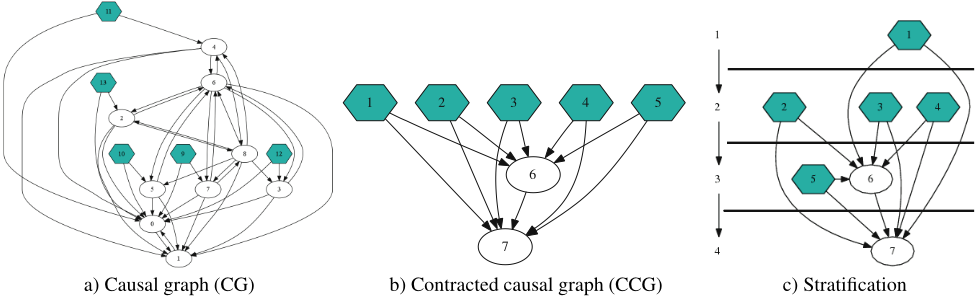
Intuitively, the nodes in the CG are state variables and the arrows in CG describe the dependency relationships between variables. If the CG contains an arc fromxi to xj , then a value change of xj will possibly affect the applicability of some action o that involves a transition of xi. Figure 1a shows the CG of an instance (Truck-02) of the Truck planning domain used in the 5th International Planning Competition (IPC5). State variables that define the goal state are in darker color.
3 Stratification of Planning Problems
Now we propose our stratification analysis. Given a SAS+ task, usually its CG is not acyclic, which leads to cyclic causal dependencies among some of (but often not all) the state variables. We propose a strongly connected component analysis on CG.
A directed graph is called strongly connected if there is a path from each vertex in the graph to every other vertex. For a directed graph, a strongly connected component (SCC)
is a maximal strongly connected subgraph. A directed graph can be uniquely decomposed into several SCCs. A partition of a set X is a set of nonempty subsets of X such that every element x in X is in exactly one of these subsets.
Definition 2 (Component Set). Given a SAS+ planning task Π and its causal graph CG(Π) = (X, E), the component set M(Π) is the partition of X such that all the elements in each m ∈ M(Π) are in the same SCC of CG(Π).
Definition 3 (Contracted Graph). Given a directed graph G = (V,E), a contracted graph of G is a directed graph G′ = (V ′ ,E′ ), where each v′ ∈ V ′ is a subset of V and V ′ is a partition of V . There is an arc (v′ ,w′ ) ∈ E′ if and only if there exist v ∈ v′ and w ∈ w′ such that (v, w) ∈ E.
Definition 4 (Contracted Causal Graph (CCG)). Given a SAS+ planning task Π, its contracted causal graph CCG(Π) = (V,E) is a contracted graph of CG(Π) such that V =M(Π).
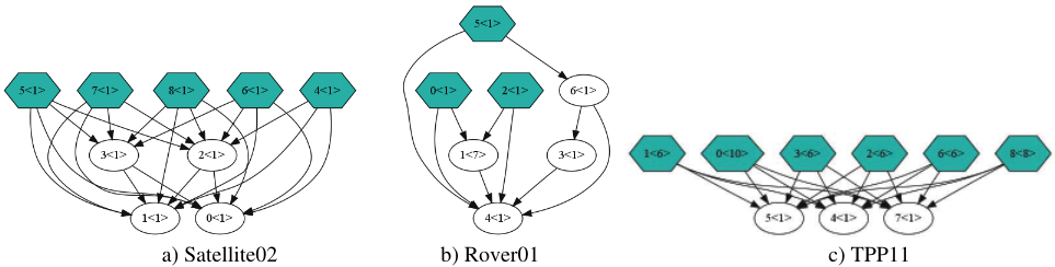
Figure 1b shows the corresponding CCG of Figure 1a. Each vertex in the CCG may contain more than one state variable. Intuitively, given the CG of a graph, we find its SCCs and contract each SCC into a vertex. The resulting graph is the CCG. Figure 2 shows the CCG of some other domains. The CCG plays the central role in our structural analysis. It has an important property.
Proposition 1. For any SAS+ planning task Π, CCG(Π) is a directed acyclic graph (DAG).
The above statement is true because if the CCG contains a cycle, then all the vertices on that cycle are strongly connected and should be contracted into one SCC. Therefore, we see that although there are dependency cycles in the CG, there is no cycle after we contract each SCC to one vertex. A topological sort on the CCG gives an list of the SCCs, ordered by dependency relations. Stratification can be viewed as a generalization of topological sort.
Definition 5 (Stratification). Given a DAG G = (V,E), a stratification Str(G) of G is a tuple (U,L), where U = {u1, · · · , uk} is a partition of V . U satisfies that there do not exist i, j, 1 ≤ i < j ≤ k, vi ∈ ui, and vj ∈ uj such that (vj, vi) ∈ E. The function L : V ↦→ N+ is called the layer function. L(v) = k for any v ∈ V and v ∈ uk.
The stratification of a DAG G = (V,E) is not unique. A stratification Str(G) = (U, L) is called a k-stratification if |U| = k. The upper bound of k is |V |. When k = |V |, U must be a topological sort of V .
Definition 6 (Stratification of a SAS+ Task). Given a SAS+ planning task Π, a stratification of Π, denoted by Str(Π), is a stratification of CCG(Π).
Intuitively, a stratification of a CCG gives the flexibility to cluster state variables while pertaining to the topological order. There can be one-way dependency or no dependency, but no two-way dependency, between any two state variables at different layers under a stratification.
Figure 1c shows an example of stratification of the Truck02 problem. Each SCC in Figure 1b is now assigned a layer and the topological order is maintained in the stratification. Basicly, the requirement is that there is no arrow pointing from a larger-numbered layer to a smaller-numbered one.
The stratification defines the layer function for any state variable x ∈ X. Based on that, we can define the layer function L(o) for each action o ∈ O.
Definition 7 (Action Layer). For a SAS+ task Π, given a stratification Str(Π) = (U, L), for an action o ∈ O, L(o) is defined as L(x), for an arbitrary x ∈ trans(o), if trans(o) is nonempty; and L(o) = ∞ if trans(o) = ∅.
We prove that L(o) is well-defined by showing that all x ∈ trans(o) has the same L(x), for any action o ∈ O.
Proposition 2. For a SAS+ task Π, for an action o ∈ O with trans(o) ̸= ∅, we have L(xi) = L(xj ), ∀xi, xj ∈ trans(o).
Proof. Since xj ∈ trans(o) ⊆ dep(o) and xi ∈ trans(o), by Definition 1, there is an arc from xj to xi in CG(Π). Similarly, xi ∈ trans(o) ⊆ dep(o) and xj ∈ trans(o), an arc exists from xi to xj in CG(Π). This implies that xi and xj are strongly connected in CG(Π) and are elements in a same vertex of CCG(Π). By Definition 5, we have L(xi) = L(xj ).
4 Stratified Planning Algorithm
Now we propose our stratified planning algorithm. In fact, it is not a standalone algorithm but rather a space reduction method that can be combined with other search algorithms. It reduces the number of actions that need to be expanded at each state.
We outline stratified planning in Algorithm 1. The input is a SAS+ task Π and a stratification Str(Π). It is a general framework where the open list can be implemented as a stack, queue or priority queue. The open list contains a list of states that are generated but not expanded.
Input: A SAS+ planning task Π and a stratification Str(Π) = (U, L) Output: A solution plan closed ← an empty set; 1 insert the initial AS pair (no-op,sI) to open; 2 while open is not empty do 3 (a, s) ← remove-next(open); 4 if s is a goal state then return solution; 5 if s is not in closed then 6 add s to closed; 7 Ψ(a, s, L) = stratified expansion(a, s, L) ; 8 open ← open∪ Ψ(a, s, L); 9Definition 8. For the purpose of stratified planning, for each generated state s, we record an action-state (AS) pair (a, s) in the open list, where a is the action that leads to s during the search. a is called the leading action of s.
Each time during the search, a remove-next() operation fetches one AS pair (a, s) from open, checks if the state s is a goal state or is in the closed list. If not, the stratified expansion() operation will generate a set of AS pairs (b, s′ ) to be inserted to open, where s′ is the resulting state of applying b to s, i.e. s′ = apply(s, b).
The difference between stratified planning and a standard search is that, in standard search, we will expand all the actions that are applicable at s, while stratified expansion() may not expand every applicable action.
Since the initial state sI has no leading action, a special action no-op is defined as its leading action and its layer is defined as 0.
Definition 9 (Follow-up Action). For a SAS+ task Π, for two actions a, b ∈ O, b is a follow-up action of a (denoted as a ▷ b) if aff(a)∩dep(b) ̸= ∅ or aff(a)∩aff(b) ̸= ∅. Any action is a follow-up action of no-op.
Given this definition, we can describe the stratified expansion() operation, shown in Algorithm 2. Given a stratification Str(Π) = (U,L), the procedure of stratified expansion() is quite simple. For any AS pair (a, s) to be expanded, for each action b ∈ O that is applicable at s, we consider two cases.
- If L(b) ≥ L(a), we expand b.
- If L(b) < L(a), we expand b only if b is a follow-up action of a (a ▷ b).
For any AS pair (a, s), all the AS pairs expanded by stratified expansion() forms the set Ψ(a, s, L).
5 Theoretical Analysis
In this section, we show that stratified planning search preserves the completeness and optimality property of the original search strategy, decided by the implementation of the open list and the evaluation function. For example, if open is a priority queue and the evaluation function is admissible, then the original search, with a full expansion at each state, is both complete and optimal.
Input: An AS pair (a, s) and the L function Output: The set Ψ(a, s, L) of successor AS pairs Ψ ← ∅; 1 foreach applicable action b at s do 2 if L(b) ≥ L(a) then 3 compute s′ = apply(s, b); 4 Ψ ← Ψ ∪ {(b, s′ )} ; 5 else if a ▷ b then 6 compute s′ = apply(s, b); 7 Ψ ← Ψ ∪ {(b, s′ )} ; 8 9 end 10 return Ψ ; 11Definition 10 (Valid Path). For a SAS+ task Π and a state s0, a sequence of actions p = (o1, . . . , on) is a valid path if, let si = apply(si-1, oi), i = 1, . . . , n, oi is applicable at si-1 for i = 1, . . . , n. We also say that applying p to s results in the state sn.
Definition 11 (Stratified Path). For a SAS+ task Π, for a stratification str(Π) = (U, L) and a state s0, a sequence of actions p = (o1, . . . , on) is a stratified path if it is a valid path and, let si = apply(si-1, oi), i = 1, . . . , n, (oi, si) ∈ Ψ(oi-1, si-1, L) for i = 1, . . . , n, where o0 = no-op.
Intuitively, a stratified path is a sequence of actions that can possibly be generated by the stratified search.
Lemma 1. For a SAS+ task Π, a stratification str(Π) = (U,L) and a state s0, for any valid path p = (a1, . . . , an), if there exists 2 ≤ i ≤ n, such that L(ai) < L(ai-1) and that ai is not a follow-up action of ai-1, then p′ = (a1, . . . , ai-2, ai, ai-1, ai+1, . . . , an) is also a valid path and leads to the same state from s0 as p does.
Proof. Let sj = apply(sj-1, aj), j = 1, · · · , n. Since ai is not a follow-up action of ai-1, according to Definition 9, eff(ai-1) contains no assignment in pre(ai). Therefore, since ai is applicable at si-1, which is apply(si-2, ai-1), we know ai is also applicable at si-2.
Since L(ai) < L(ai-1), the SCC in CCG(Π) that contains ai-1 has no dependencies on the SCC that contains ai. Therefore, eff(ai) contains no assignment in pre(ai-1). Since the variable assignments in pre(ai-1) are satisfied at si-2, it is also satisfied at s′ = apply(si-2, ai).
From the above, we see that (ai, ai-1) is an applicable action sequence at si-2. Further, since ai is not a follow-up action of ai-1, we have that aff(ai) ∩ aff(ai-1) = ∅. Hence, applying (ai, ai-1) to si-2 leads to the same state as applying (ai-1, ai), which is si. Therefore, p′ is a valid path from s0 and leads to the same state as p does.
Theorem 1. Given a SAS+ planning task Π and a stratification Str(Π), for any state s0 and any valid path pa = (a1, . . . , an) from s0, there exists a stratified path pb = (b1, . . . , bn) from s0 such that pa and pb result in the same state when applied to s0.
Proof. We prove by induction on the number of actions. When n = 1, since the only action in the path p is a follow-up action of no-op, p is also a stratified path. Now we assume the proposition is true for n = k, k ≥ 1 and prove the case when n = k + 1.
For a valid path p0 = (a1, . . . , ak+1), by our induction hypothesis, we can permute the first k actions to obtain a stratified path (a11, . . . , a1k ).
Now we consider a new path p1 = (a11 , . . . , a1k , ak+1). If we have L(ak+1) ≤ L(a1k ), or L(ak+1) > L(a1k ) and ak+1 is a follow-up action of a1k , then p1 is already a stratified path.
Now we focus on the case when L(ak+1) > L(a1k ) and ak+1 is not a follow-up action of a1k . Consider a new path p2 = (a11, . . . , a1k-1 , ak+1, a1k ). From Lemma 1, we know that p2 is a valid path leading to the same state as p1 does.
By our induction hypothesis, we can permute the first k actions of p2 to obtain a stratified path (a21, . . . , a2k ). Define p3 = (a21, . . . , a2k , a1k ).
Comparing p2 and p3 , we know that L(ak+1) > L(a1k ), namely, the level of the last action in p2 is strictly larger than that in p3 . We can repeat the above process to generate p4 , p5 , · · · , as long as pj , (j ∈ Z +) is not a stratified path. For each pj , the first k actions is a stratified path. Also, every pj is a valid path that leads to the same state as p0 does.
Since we know that the level of the last action in pj is monotonically decreasing as j increases, such a process must stop in a finite number of iterations. Suppose it stops at pm = (a′1 , . . . , a′k , a′k+1 ),m ≥ 1. We must have that L(a′k+1 ) ≤ L(a′k ), or L(a′k+1 ) > L(a′k ) and a′k+1 is a follow-up action of a′k . Hence pm is a stratified path and the induction step is proved.
Theorem 2. For a SAS+ task, a complete search is still complete when combined with stratified expansion(), and an optimal search is still optimal when combined with stratified expansion().
Proof. For any search algorithm, we define its search graph as a graph where each vertex is a state and there is an arc from s to s′ if and only if s′ is expanded as a successor state of s during the search. For a complete search, if it can find a solution path p in the original search graph, then according to Theorem 1, there is another path p′ in the search graph of the stratified search. Therefore, the complete search combined with stratified expansion() will find p′ .
If a search is optimal, then when it is combined with stratified expansion(), it will find an optimal path p′ in the search graph of the stratified search. According to Theorem 1, if the length of the optimal path in the original search graph is n, there must exist a path in the search graph of the stratified search with length n. Hence, the length of p′ is n and the new search is still optimal.
6 Experimental Results
We test on STRIPS problems in the recent International Planning Competitions (IPCs). We implement our stratification analysis and stratified search on top the Fast Downward planner [Helmert, 2006] which gives SAS+ encoding of planning problems. We still use the causal graph heuristic and only modify the state expansion part. On a PC with a 2.0 GHz Xeon CPU and 2GB memory, we set a time limit of 300 seconds for all problem instances.
| ID | Fast Downward | ∞-stratification | 2-stratification | |||
|---|---|---|---|---|---|---|
| Nodes | Time | Nodes | Time | Nodes | Time | |
| zenotravel1 | 10 | 0 | 5 | 0 | 5 | 0 |
| zenotravel1 | 122 | 0 | 23 | 0 | 23 | 0 |
| zenotravel3 | 723 | 0 | 236 | 0 | 236 | 0 |
| zenotravel4 | 455 | 0 | 194 | 0 | 194 | 0 |
| zenotravel5 | 884 | 0 | 479 | 0 | 479 | 0 |
| zenotravel6 | 1895 | 0 | 785 | 0 | 785 | 0 |
| zenotravel7 | 1468 | 0 | 883 | 0 | 883 | 0 |
| zenotravel8 | 1795 | 0.04 | 1828 | 0.02 | 1828 | 0.02 |
| zenotravel9 | 2017 | 0.04 | 2938 | 0.04 | 2938 | 0.04 |
| zenotravel10 | 4218 | 0.05 | 8708 | 0.04 | 8708 | 0.04 |
| zenotravel11 | 3485 | 0.02 | 3429 | 0.02 | 3429 | 0.02 |
| zenotravel12 | 5002 | 0.06 | 7671 | 0.04 | 7671 | 0.04 |
| zenotravel13 | 9654 | 0.07 | 6911 | 0.12 | 6911 | 0.12 |
| zenotravel14 | 495266 | 0.26 | 49623 | 0.18 | 49623 | 0.18 |
| zenotravel15 | 23853 | 0.52 | 1254 | 0.39 | 1254 | 0.45 |
| drivelog1 | 355 | 0 | 51 | 0 | 152 | 0 |
| drivelog2 | 1450 | 0 | 633 | 0.01 | 743 | 0.01 |
| drivelog3 | 774 | 0 | 297 | 0.01 | 433 | 0.01 |
| drivelog4 | 4692 | 0.01 | 1549 | 0.03 | 3454 | 0.02 |
| drivelog5 | 2879 | 0.01 | 576 | 0.01 | 957 | 0.01 |
| drivelog6 | 2394 | 0 | 577 | 0 | 1442 | 0.01 |
| drivelog7 | 1707 | 0.02 | 4341 | 0.03 | 1948 | 0.01 |
| drivelog8 | 531 | 0 | 57006 | 0.35 | 4372 | 0.02 |
| drivelog9 | 18920 | 0.02 | 3808 | 0.03 | 26991 | 0.24 |
| drivelog10 | 10356 | 0.02 | 4317 | 0.04 | 8965 | 0.07 |
| drivelog11 | 3755 | 0.05 | 2435 | 0.04 | 3616 | 0.06 |
| drivelog12 | 64714 | 0.31 | 21252 | 0.28 | 135518 | 2.18 |
| drivelog13 | 10995 | 0.13 | 5659 | 0.14 | 9333 | 0.22 |
| drivelog14 | 14344 | 0.06 | 3195 | 0.1 | 7388 | 0.21 |
| drivelog15 | 140305 | 1.25 | 14371 | 1.39 | 14369 | 0.79 |
| drivelog16 | 1554010 | 44.49 | 180020 | 29.39 | - | - |
| drivelog17 | 2218657 | 51.33 | 860136 | 33.81 | 3986057 | 167.69 |
In practice, how to determine the granularity of stratification is an important issue. We test two extremal cases in our experiments. On one extreme, we test ∞-stratification, which performs a topological sort on the CCG and treats each SCC as a layer. This represents the finest granularity of stratification. On the other extreme, we test 2-stratification, which partitions the CCG into two layers and represents the coarsest granularity of stratification. We also implement a factor γ, 0 < γ < 1 for 2-stratification, which specifies the ratio of the number of state variables in Layer 1 to the total number of state variables. We topologically sort the CCG and find the dividing point that gives a ratio closest to γ. We use γ = 0.7 in our experiments.
The results are shown in Tables 1 and 2. We did not include the domains, such as pipesworld and freecell, where the CG is only one SCC and cannot be stratified. We can see that both ∞-stratification and 2-stratification can give reduction for most problem instances. The reduction of the number of generated nodes can be more than an order of magnitude. Comparing ∞-stratification to 2-stratification, we see that they give similar performance. Despite the reduction in number of generated nodes, the CPU time reduction is more modest. This is due to the fact that our preliminary implementation is not efficient. For example, we check whether an action is a follow-up action of another one at each state, although a preprocessing phase will save much time. We will develop more efficient implementations in our future work.
7 Discussions
The idea of stratified planning can be explained by looking at a simple 2-stratification. In a 2-stratification, all the state variables are divided into two groups, U1 and U2, where U1 depends on U2. Therefore, during the search, whenever we expand an action a in U2, there are only two purposes: to transform a state in U2 to a goal state, or to provide a precondition for an action in U1. Therefore, we allow to further expand actions in U2 but do not allow actions in U1 except those directly supported by a. In other words, we do not expand any action in U1 that is not a follow-up action of a because it is a "loose" partial order that can be pruned.
From the above, we see that stratified search can avoid redundant orderings between ancestor/offspring SCCs. Besides that, another source of reduction is that stratified planning imposes certain partial orders between sibling SCCs. For example, in Figure 1b, the SCCs numbered 1 to 5 are siblings in the CCG. However, after we stratify the CCG as in Figure 1c, we impose certain partial orders. For example, we are forced to place actions in SCC 1 before SCC 5 whenever possible. Such a reduction can be significant for many domains.
Acknowledgement
This work is supported by NSF grant IIS-0713109, a DOE ECPI award, and a Microsoft Research New Faculty Fellowship.
@inproceedings{ijcai2009p278,
  title     = {Stratified Planning},
  author    = {Chen, Yixin and Xu, You and Yao, Guohui},
  booktitle = {Proceedings of the Twenty-First International Joint Conference on
               Artificial Intelligence, {IJCAI-09}},
  publisher = {International Joint Conferences on Artificial Intelligence},
  editor    = {Craig Boutilier},
  pages     = {1665--1669},
  year      = {2009},
  url       = {https://ijcai.org/proceedings/2009/278},
}
TY - CPAPER TI - Stratified Planning AU - Chen, Yixin AU - Xu, You AU - Yao, Guohui T2 - Proceedings of the Twenty-First International Joint Conference on Artificial Intelligence, IJCAI-09 PB - International Joint Conferences on Artificial Intelligence PY - 2009 SP - 1665 EP - 1669 UR - https://ijcai.org/proceedings/2009/278 ER -Copied
Machine-readable versions of this paper, for tools and AI agents:





