
Completeness and Optimality Preserving Reduction for Planning
Proceedings of the Twenty-First International Joint Conference on Artificial Intelligence. Pages 1659-1663.
© 2009 International Joint Conferences on Artificial Intelligence
Abstract
Traditional AI search methods search in a state space typically modelled as a directed graph. Prohibitively large sizes of state space graphs make complete or optimal search expensive. A key observation, as exemplified by the SAS+ formalism for planning, is that most commonly a state-space graph can be decomposed into subgraphs, linked by constraints. We propose a novel space reduction algorithm that exploits such structure. The result reveals that standard search algorithms may explore many redundant paths. Our method provides an automatic way to remove such redundancy. At each state, we expand only the subgraphs within a dependency closure satisfying certain sufficient conditions instead of all the subgraphs. Theoretically we prove that the proposed algorithm is completeness-preserving as well as optimality-preserving. We show that our reduction method can significantly reduce the search cost on a collection of planning domains.Yixin Chen, Guohui Yao
- [Amir & Engelhardt, 2003] Amir, E., and Engelhardt, B. 2003. Factored planning. In Proc. IJCAI.
- [Bäckström & Nebel, 1995] Bäckström, C., and Nebel, B. 1995. Complexity results for SAS+ planning. Compu- tational Intelligence 11:17-29. IJCAI
- [Bonet & Geffner, 2001] Bonet, B., and Geffner, H. 2001. Planning as heuristic search. Artificial Intelligence 129:5- 33.
- [Brafman & Domshlak, 2006] Brafman, R., and Domshlak, C. 2006. Factored planning: How, when, and when not. In Proc. AAAI.
- [Fox & Long, 1999] Fox, M., and Long, D. 1999. The detec- tion and exploitation of symmetry in planning problems. In Proc. IJCAI. IJCAI
- [Helmert & Röger, 2008] Helmert, M., and Röger, G. 2008. How good is almost perfect. In Proc. AAAI.
- [Helmert, Haslum, & Hoffmann, 2007] Helmert, M.; Haslum, P.; and Hoffmann, J. 2007. Flexible abstraction heuristics for optimal sequential planning. In Proc. ICAPS.
- [Helmert, 2006] Helmert, M. 2006. The Fast Downward planning system. Journal of Artificial Intelligence Re- search 26:191-246.
- [Jonsson & Bäckström, 1998] Jonsson, P., and Bäckström, C. 1998. State-variable planning under structural restric- tions: Algorithms and complexity. Artificial Intelligence 100(1-2):125-176.
References were extracted automatically from the PDF and may contain errors.
Full text extracted automatically from the PDF; figures, tables and equations may differ. The PDF is the version of record.
1 Introduction
State-space search is a fundamental and pervasive approach for AI. The state space is typically modelled as a directed graph. A cost can be associated with each edge in the graph and the search tries to identify the path with the minimum total cost from an initial state to a goal state.
A key observation that motivates this paper is that most often the state-space is not a random graph. Rather, in most domains, the state space graph can be viewed as part of the Cartesian product of multiple smaller subgraphs. In SAS+ formalism [B¨ackstr ¨om & Nebel, 1995; Jonsson & B¨ackstr ¨om, 1998] of planning, a state is represented by the assignments to a set of multi-valued variables, and the state-space graph is derived from the Cartesian product of the domain transition graphs (DTGs), one for each variable.
The key question is, if a state-space graph can be decomposed as the Cartesian product of subgraphs, can we make the search faster by exploiting such structure?
∗Ph.D. candidate affiliated with Shandong University.
Guohui Yao ∗
Department of Computer Science Washington University yaog@cse.wustl.edu
Given the large size of the search space, exploiting decomposition of planning domains has long been of interests to planning researchers. There are several lines of existing work:
- The automated hierarchical planning [Knoblock, 1994; Lansky & Getoor, 1995] methods utilize hierarchical factoring of planning domains, but they typically do not scale well since they require extensive backtracking across subdomains.
- To avoid the cost of backtracking, the factored planning approach [Amir & Engelhardt, 2003; Brafman & Domshlak, 2006] finds all the subplans for each subproblem before merging some of them into one solution plan. However, as enumerating all subplans requires huge memory and time complexity, the practicability of factored planning has not been fully established [Kelareva et al., 2007]. Our own empirical results suggest that the cost of factored planning can be exceedingly high. Also, the iterative deepening scheme that increments the length of the subplans poses additional complexity and compromises optimality.
- Decomposition of planning domains has also been used to derive better heuristics [Helmert, 2006; Helmert, Haslum, & Hoffmann, 2007] inside a heuristic search planner. However, as revealed by recent work [Helmert & R¨oger, 2008], an admissible search with even almost perfect heuristics may still have exponential complexity. Hence, it is important to improve other components of the search algorithm that are orthogonal to the design of better heuristics.
The main contribution of this paper is a completenesspreserving reduction technique, the expansion core (EC) method, that can be combined with search algorithms on SAS+ planning domains. The key idea of EC is that, by restricting the set of actions to be expanded at each state, we are in effect removing a lot of redundant ordering of actions. For example, for a given state s, if for any solution path from s that places an action a before b, there exists another solution path from s that places b before a, then it reduces the search space to remove the ordering a → b and only consider those plans that place b before a.
Technically, the EC method modifies the way each node is expanded during the search. When searching in a Cartesian product of subgraphs, expanding a node amounts to expanding executable actions in all the subgraphs, which we reveal is often wasteful. EC expands a subset of subgraphs that form a dependency closure and still maintains the completeness and optimality of search.
The partial order based reduction idea behind EC has been studied in the model checking community to address the state space explosion problem [Valmari, 1998]. However, clean and domain-independent reduction ideas for planning are few. Symmetry detection [Fox & Long, 1999] is one such idea that can be used to reduce redundant partial orderings in planning. We discuss later that our algorithm is different from symmetry detection.
This paper is organized as follows. We first give basic definitions in Section 2. We then propose the EC method in Section 3. We report experimental results in Section 4 and give conclusions in Section 5.
2 Background
A SAS+ planning task is defined on a set of state variables X = {x1, · · · , xN}, each with a domain Dom(xi); and a set of actions O, where each action o ∈ O is a tuple (pre(o), eff(o)), where pre(o) defines some partial assignments of the state variables and eff(o) defines a set of value transitions (vi, v′i ), vi ∈ Dom(xi) ∪ {unknown}, v′i ∈ Dom(xi).
A complete assignment of the state variables is a state. We can write a state s as s = (s1, . . . , sN), where each si ∈ Dom(xi) is the assignment to variable xi. For each state s, an action o is executable if s agrees to the partial assignments in pre(o) and the first component of each element of eff(o). Applying o to s leads to a new state s′ = result(s, o) where the value of xi is changed to v′i for each (vi, v′i ) ∈ eff(o) and other state variables keep their value. result(s, o) is undefined if o is not executable at S. vi can take value from Dom(xi) or be "unknown", which means the action will lead to state v′i regardless of the value of xi. The planning task is to find an executable sequence of actions that transits a state (s0) to a partial assignment to state variables (a goal state).
A task can also specify a optimality criterion. In this paper we assume that each action has a positive cost and the task is to minimize the total action costs. Optimal search algorithms such as A∗ can optimize this preference using admissible heuristics.
Each state variable xi, i = 1, · · · ,N is associated with a domain transition graph (DTG) Gi, a directed graph with vertex set V (Gi) = Dom(xi) and edge set E(Gi). An edge (vi, v′i ) belongs to E(Gi) if and only if there is an action o with (vi, v′i ) ∈ eff(o), in which case we say that o is associated with the edge ei = (vi, v′i ) (denoted as o ⊢ ei). A DTG Gi is goal-related if the partial assignments that define the goal states include an assignment in Gi.
Definition 1 An action o is associated with a DTG Gi (denoted as o ⊢ Gi) if o is associated with any edge in Gi.
3 Expansion Core (EC) Method
Now we propose our search space reduction method. We characterize standard search algorithms by Algorithm 1. Different search algorithms differ by the remove-first() operation which fetches one node from the open list. Algorithm 1 is depth-first search (DFS) when open is a FILO queue, breadth
Algorithm1: State space search
Input: State space graph G Output: p, an optimal solution path closed ← an empty set; 1 insert the initial state s0 into open; 2 while open is not empty do 3 s ← remove-first(open); 4 if s is a goal state then process solution path(s); 5 if s is not in closed then 6 add s to closed; 7 open ← insert(expand(s), open); 8first search (BFS) when open is a FIFO queue, best-first search (including A∗ ) when open is a priority queue ordered by an evaluation function.
We define a reduction method as a method to expand only a subset of the set expand(s) in Algorithm 1 for each state s during the search. Normally a reduction method can be combined with any implementation of remove-first() and any heuristic function to form various algorithms. While the strategies for remove-first() and the design of heuristic functions have been heavily studied, the possible reduction of expand() has been rarely studied in planning.
The standard definition of expand(s), for a state s in a SAS+ task, is the set of states reachable from s by executing one action. Let the set of executable actions at s be exec(s), we have expand(s) = {result(s, o)|o ∈ exec(s)}.
Definition 2 For a SAS+ task, for each DTG Gi, i = 1, . . . ,N, for a vertex v ∈ V (Gi), an edge e ∈ E(Gi) is a potential descendant edge of v (denoted as v ◁ e) if 1) Gi is goal-related and there exists a path from v to the goal state in Gi that contains e; or 2) Gi is not goal-related and e is reachable from v. A vertex w ∈ V (Gi) is a potential descendant vertex of v (denoted as v ◁w) if 1) Gi is goal-related and there exists a path from v to the goal state in Gi that contains w; or 2) Gi is not goal-related and w is reachable from v.
In a preprocessing phase, for each DTG Gi, we may decide for all vertex-edge pair (v, e), v ∈ V (Gi), e ∈ E(Gi), whether v ◁ e in time polynomial to |V (Gi)| + |E(Gi)|. The algorithm checks, for each (v, e), e = (u, w), whether v can reach u and w can reach the goal state, if any. We have v ◁ e if both can be achieved. The v ◁ w relationship of all vertex pairs can be decided similarly.
Definition 3 For a SAS+ task, for each action o ∈ O, we define need(o) as the set
need(o) = pre(o) ∪ {vi|(vi , v′i ) ∈ ef f (o)}.Intuitively, pre(o) is the set of prevailing preconditions, while need(o) is the set of all preconditions, including the second subset in the equation which we call transitional preconditions. Note that, we do not include "unknown" in need(o) since it does not really require a precondition.
Definition 4 For a SAS+ task, given a state s = (s1, · · · , sN), for any 1 ≤ i, j ≤ N, i ̸= j, we call si a potential precondition of the DTG Gj if there exist o ∈ O and ej ∈ E(Gj) such that
Definition 5 For a SAS+ task, given a state s = (s1, . . . , sN), for any 1 ≤ i, j ≤ N, i ̸= j, we call si a potential dependent of the DTG Gj if there exists o ∈ O, ei = (si, s′i ) ∈ E(Gi) and wj ∈ V (Gj ) such that
Definition 6 For a SAS+ task, for a state s = (s1, . . . , sN), its potential dependency graph PDG(s) is a directed graph in which each DTG Gi, i = 1, · · · ,N corresponds to a vertex, and there is an edge from Gi to Gj , i ̸= j, if and only if si is a potential precondition or potential dependent of Gj .
Definition 7 For a directed graph H, a subset C of V (H) is a dependency closure if there do not exist v ∈ C and w ∈ V (H) - C such that (v, w) ∈ E(H).
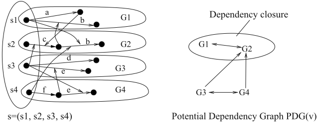
Figure 1 illustrates the above definitions. In PDG(s), G1 points to G2 as s1 is a potential precondition of G2 and G2 points to G1 as s2 is a potential dependent of G1. We also see that G1 and G2 form a dependency closure of PDG(s).
Given PDG(s), we first find the strongly connected components (SCCs) of it. If each SCC is contracted to a single vertex, the resulting graph is a directed acyclic graph S. We observe that each SCC in S with a zero out-degree forms a dependency closure.
The expansion core (EC) method can be described as follows. In the expand(s) operation, instead of expanding actions in all the DTGs, we only expand actions in DTGs that belong to a dependency closure of PDG(s) under the condition that not all DTGs in the dependency closure are at a goal state. The operation is described as follows.
Definition 8 The EC method modifies the expand(s) operation in Algorithm 1 to:
where C(s) ⊆ {1, · · · ,N} is an index set satisfying:
- The DTGs {Gi, i ∈ C(s)} form a dependency closure in PDG(s); and
2) there exists i ∈ C(s) such that Gi is goal-related and si is not the goal state in Gi.
The set C(s) can always be found for any non-goal state s since PDG(s) itself is always such a dependency closure. If there are more than one such closure, theoretically any dependency closure satisfying the above conditions can be used in EC without losing completeness. In practice, we choose the one with the minimum number of DTGs.
3.1 Theoretical analysis
We define some generic properties of reduction methods before analyzing the EC method. For a SAS+ task, its statespace graph is a directed graph G in which each state s is a vertex and there is an edge (s, s′ ) if and only if there exists an action o such that result(s, o) = s′ . For a reduction method, we can get a reduced state-space graph in which there is an edge (s, s′ ) only if s′ will be expanded as a child of s by the reduction method. For EC, the EC-reduced state-space graph Gr is a directed graph in which each state s is a vertex and there is an edge (s, s′ ) if and only if s′ ∈ expandr(s).
For a SAS+ task, a solution sequence in a state-space graph G is a pair (s0 , p), where s0 is a non-goal state, p = (a1, . . . , ak) is a sequence of actions, and, let si = result(si-1 , ai), i = 1, . . . , k, (si-1 , si ) is an edge in G for i = 1, . . . , k and sk is a goal state.
Definition 9 A reduction method is completeness-preserving if for any solution sequence (s0 , p) in the state-space graph, there also exists a solution sequence (s0 , p′ ) in the reduced state-space graph.
Definition 10 A reduction method is cost-preserving (respectively, action-preserving) if, for any solution sequence (s0 , p) in the state-space graph, there also exists a solution sequence (s0 , p′ ) in the reduced state-space graph satisfying that p′ has the same total action cost as p does (respectively, p′ is a re-ordering of the actions in p).
Clearly, action-preserving implies cost-preserving, which implies completeness-preserving.
Theorem 1 The EC method is action-preserving.
Proof. We prove that for any solution sequence (s0 , p) in the state-space graph G, there exists a solution sequence (s0 , p′ ) in the EC-reduced state-space graph Gr such that p′ is a reordering of actions in p. We prove this fact by induction on k, the length of the path p. In our proof, sij denotes the value of the DTGGj at state si .
When k = 1, let a be the only action in p, for any goalrelated DTG Gi such that s0i is not the goal in Gi, we must have a ⊢ Gi. According to the second condition in Definition 8, since C(s0 ) must include the index of a goal-related DTG whose state is not the goal (let it be j), we have that a ⊢ Gj and that result(s0, a) ∈ expandr(s0 ). Thus, (s0 , p) is also a solution sequence in Gr. The EC method is actionpreserving in the base case.
When k > 1, consider a solution sequence (s0 , p) in G: p = (a1, . . . , ak). Let si = result(si-1 , ai), i = 1, . . . , k. We consider two cases.
a) If there exists l ∈ C(s0 ) such that a1 ⊢ Gl, then s1 ∈ expandr(s0 ) and (s0 , s1 ) is in Gr. Let p∗ = (a2 , · · · , ak ), then (s1 , p∗ ) is also a solution sequence in G. According the induction assumption, there exists a solution sequence (s1 , p∗∗ ) in Gr such that p∗∗ is a re-ordering of the actions in p∗. Therefore, a1 followed by p∗∗ is a solution sequence (starting from s0 ) in Gr and is a re-ordering of p.
b) If there exists no l ∈ C(s0 ) such that a1 ⊢ Gl, let aj be the first action in p such that there exists m ∈ C(s0 ) and aj ⊢ Gm. Such an action must exist because of the second condition in Definition 8. Consider the sequence p∗ = (aj, a1, · · · , aj-1, aj+1, · · · , ak).
For any h ∈ {1, · · · ,N} such that s0h ∈ need(aj), Gm will point to Gh in PDG(s0 ) since s0m is a potential dependent of Gh. Since m ∈ C(s0 ), we have h ∈ C(s0 ). Hence, none of the preconditions of aj is in Gi, i /∈ C(s0 ). On the other hand, s0i = sj-1 i , ∀i ∈ C(s0 ) and all the preconditions of aj are satisfied at at sj-1 . Thus, all the preconditions of aj are satisfied at s0 and aj can be executed at s0 .
Let s′ = result(s0 , aj). We know (a1, · · · , aj-1) is an executable action sequence starting from s′ . This is true because none of a1, · · · , aj-1 has a precondition in a DTG that aj is associated with (otherwise Gm will point to that DTG, forcing that DTG to be in C(s0 ), which is a contradiction to the way we choose aj. Therefore, moving aj before (a1, · · · , aj-1) will not make any of their preconditions unsatisfied. Further, since executing (a1, · · · , aj) and (aj, a1, · · · , aj-1) froms0 lead to the same state, aj+1, · · · , ak is an executable action sequence after (aj, a1, · · · , aj-1) is executed.
From the above, we see (s0 , p∗ ) is a solution sequence in G. Let p∗∗ = (a1, · · · , aj-1, aj+1, · · · , ak), (s′ , p∗∗ ) is a solution sequence in G. From the induction assumption, we know there is a sequence p′ which is a re-ordering of p∗∗ , such that (s′ , p′ ) is a solution sequence in Gr. Since s′ ∈ expandr(s0 ), we have that aj followed by p′ is a solution sequence from s0 and is a re-ordering of p∗ , which is a reordering of p. Thus, the ECmethod is action-preserving. ■
Since the EC method is action-preserving, it is also costpreserving and completeness-preserving.
Example. An example is shown in Figures 2 and 3. Figure 2 shows a SAS+ task, where a1 is the initial state and e5 is the goal state. In Figure 3, a) and b) show the original and EC-reduced search space, respectively. We see that EC significantly reduces the space. For example, at node a1, since a is not a potential dependent or precondition of G2, we can only expand G1 instead of expanding both DTGs. As another example, at b4, 4 is a potential precondition of G1, but b is not a potential dependent or precondition of G2. So at b4, G1 is a dependency closure and we only expand G1. In our case, there is no executable action in G1 at b4 and we can safely conclude that b4 cannot reach the goal although there is an executable action in G2. The reason is that, if expanding G2 can make true certain preconditions for actions in G1, then b would be a potential dependent of G2 and G2 would be in the dependency closure.
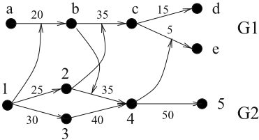
In the original space, the optimal cost 145. In the ECreduced space we can still find an optimal path (in bold) with cost 145, which validates the correctness of the EC method.
EC allows us to search on the reduced graph Gr. Since expandr() is always a subset of expand(), we have |E(Gr)| ≤ |E(G)|. Further, although |V (Gr)| = |V (G)|, the vertices reachable from the initial state may be much fewer in Gr, as shown in Figures 3. The number of vertices is reduced from 16 to 10 and number of edges from 21 to 9.
Theorem 2 For a SAS+ task, a complete search with the EC method is still complete; an optimal search with the EC method is still optimal.
Proof. Since the EC method is completeness-preserving, if there is a solution path in G, there is also a solution path in Gr, which will be found by a complete search with the EC method. Since the EC method is cost-preserving, an optimal search with the EC method will find an optimal path in Gr, which is also an optimal path in G. ■
Theorem 3 For an admissible A∗ search on a SAS+ task, for nodes with f < f ∗ where f ∗ is the cost of the optimal plan, the A∗ search with the EC method expands no more such nodes than the original A∗ search does.
Theorem 3 can be easily seen. For each node v that A∗ with the EC method expands, if its f = g + h is less than the optimal cost, it must also be expanded by the original A∗ . A node with f < f ∗ will always be expanded by A∗ but may not be expanded when EC is used, as shown in Figure 3. Hence, an A∗ search with the EC method is guaranteed to expand at most as many nodes as A∗ except possibly through tie-breaking among nodes with f = f ∗.
For inadmissible search, although it is hard to give a similar result as Theorem 3, empirical study shows that EC typically also reduces the search cost.
We give a couple of additional comments below.

Symmetry. Symmetry detection is another way for reducing the search space [Fox & Long, 1999]. From the view of node expansion on a SAS+ formalism for planning, we can see that symmetry removal is different from EC. For example, consider a domain with three objects A1, A2, and B, where A1 and A2 are symmetric, and B has no interaction with A1 or A2. In this case, symmetry removal will expand DTGs for (A1 and B) or (A2 and B), whereas EC will only expand the DTG for B since the DTG for B forms a dependency closure. Intuitively, symmetric removal finds that it is not important whether A1 or A2 is used since they are symmetric, whereas EC finds that it is not important whether B is used before or after Ai, i = 1, 2 since there is no dependency.
Limitations. EC is most effective for the case where the DTGs are "directional" and the inter-DTG dependencies are not dense. It may not be useful for problems where the DTGs are strongly connected and there is a high degree of interDTG dependencies. For example, it is not useful for the 15puzzle where each piece corresponds to a DTG which is a clique. Since each move excludes any other piece on the target position, any action in a DTG depends on all the other DTGs. Thus, the potential dependency graph is a clique for all the states and EC cannot give any reduction.
4 Experimental Results
We test on STRIPS problems in the recent International Planning Competitions (IPCs): IPC3, IPC4, and IPC5. We use a preprocessor in Fast Downward (FD) [Helmert, 2006] to convert a STRIPS problem into a SAS+ instance with multiple DTGs. Each instance is assigned 300 seconds to solve.
In our implementation, to save time for computing the expandr() set for each state, we use a preprocessing phase to precompute some reachability information of those DTGs that do not depend on others. For every pair (vi,Gj), vi ∈ Dom(xi), we precompute if vi is a potential dependent or potential precondition of Gj .
Table 1 shows the results of applying EC to an A∗ search with the admissible HSP heuristic [Bonet & Geffner, 2001]. Table 2 shows the results of applying EC to the Fast Downward planner with the casual graph (CG) heuristic and without the helper action heuristic. Both HSP and HSP+EC give the same plan length since they are both optimal (according to Theorem 2). For CG and CG+EC, their solution lengths are similar. For instances in Table 2, they give the same plan length in 21% of the cases, CG gives shorter plans in 41% of the cases, and CG+EC gives shorter plans in 38% of the cases.
From the tables, we see that EC can reduce the search cost, in terms of time and the number of generated nodes, significantly for most domains, although the degree of reduction is domain-dependent. The numbers of expanded nodes are also largely reduced, although not shown in the table due to space limit. The reduction is very significant for some domains and is more than 100 times for some instances. We do not show results on three domains where the EC method gives no reduction: pipesworld, freecell, and storage.
To gain some insights on why the EC method performs better for certain domains, we examine the causal graph (CG) [Helmert, 2006] of each domain. The CG is a graph where each vertex is a DTG and the edges represent dependencies among DTGs. For each CG, we find its strongly connected components (SCCs) and contract each SCC into a vertex. We find that for domains where EC is very effective (such as rovers and satellite), their CG can be decomposed into multiple SCCs (for example, 9 SCCs for satellite02), while for domains where EC is not useful (such as pipesworld and freecell), their CG is just one single SCC.
From Table 1 and Table 2, we also see that the EC method gives significant reduction for both admissible (HSP) and inadmissible (CG) heuristics. It seems that the degree of reduction that EC can give is more related to the domain structure than to the quality of heuristics. We explain this observation by the following. The goal of the EC method is to avoid trying redundant partial orderings of actions. For example, at a state s, if the action orderings b → a and a → b are determined to be redundant by the EC method, then EC will choose to expand only one ordering, say a → b. Using a better heuristic may not help prune one of those two orderings. Let sa = result(s, a), sb = result(s, b), and sab = result(sa, b) = result(sb, a). Normally, we would have f(sa) ≤ f(sab) and f(sb) ≤ f(sab) if the heuristic is consistent. Hence, sa and sb will both be expanded before sab is expanded and the search will essentially try both b → a and a → b even if the heuristic is highly accurate. This is essentially the same reasoning used in [Helmert & R¨oger, 2008] to explain why an almost perfect heuristic may still lead to high search costs. The EC method is orthogonal to the design of heuristics and can reduce redundant orderings.
5 Conclusions
We have proposed EC, a completeness-preserving reduction method for SAS+ planning which provides an automatic way to reduce the search space without losing completeness and optimality. EC is a general principle for removing redundancy in search and does not require any parameter tuning.
| ID | HSP+EC | HSP | ID | HSP+EC | HSP | ||||
|---|---|---|---|---|---|---|---|---|---|
| Time | Node | Time | Node | Time | Node | Time | Node | ||
| zeno02 zeno04 zeno06 | 0.01 0.16 11.11 | 93 9585 1395342 | 0.01 0.14 11.3 | 127 10215 1624301 | zeno03 zeno05 zeno07 | 0.08 1.59 11.4 | 4679 157406 1379764 | 0.08 1.55 11.69 | 5762 185715 1628619 |
| rovers01 rovers03 rovers05 | 0.01 0.05 44.51 | 949 2869 3768608 | 0.01 0.03 - | 2043 5724 - | rovers02 rovers04 rovers07 | 0.01 0.02 231.9 | 254 935 15093217 | 0.01 0.01 - | 1019 2399 - |
| rovers5-01 rovers5-03 rovers5-05 | 0.01 0.05 45.68 | 949 2869 3768608 | 0.01 0.03 - | 2043 5724 - | rovers5-02 rovers5-04 | 0.01 0.02 | 254 935 | 0.01 0.01 | 1019 2399 |
| tpp01 tpp03 tpp05 | 0.01 0.01 1.35 | 5 11 53715 | 0.01 0.01 0.34 | 8 188 72689 | tpp02 tpp04 | 0.01 0.01 | 8 14 | 0.01 0.01 | 34 1130 |
| satellite01 satellite03 | 0.01 0.54 | 367 31123 | 0.01 1.13 | 437 151351 | satellite02 satellite04 | 0.07 6.38 | 5820 781393 | 0.04 16.13 | 6724 3894047 |
| depots01 | 0.01 | 725 | 0.01 | 1000 | depots02 | 1.01 | 17613 | 1.07 0.03 | 17903 |
| pathways1 pathways3 | 0.01 1.48 | 146 47852 | 0.01 0.37 | 162 82588 | pathways2 pathways4 | 0.06 22.4 | 2600 597628 | 12.86 | 2890 2112481 |
| driverlog01 driverlog03 driverlog05 driverlog07 | 0.01 0.09 135.78 20.36 | 293 15302 14806514 1960212 | 0.01 0.09 144.22 77.76 | 373 22685 24223525 10115601 | driverlog02 driverlog04 driverlog06 | 2.32 12.87 6.22 | 192915 1430792 650872 | 1.99 26.29 8.25 | 417835 4794197 1289283 |
EC is orthogonal to and can be combined with the development of other components of search such as heuristics and search control strategies.
Acknowledgement
This work is supported by NSF grant IIS-0713109, a DOE ECPI award, and a Microsoft Research New Faculty Fellowship.
@inproceedings{ijcai2009p277,
  title     = {Completeness and Optimality Preserving Reduction for Planning},
  author    = {Chen, Yixin and Yao, Guohui},
  booktitle = {Proceedings of the Twenty-First International Joint Conference on
               Artificial Intelligence, {IJCAI-09}},
  publisher = {International Joint Conferences on Artificial Intelligence},
  editor    = {Craig Boutilier},
  pages     = {1659--1663},
  year      = {2009},
  url       = {https://ijcai.org/proceedings/2009/277},
}
TY - CPAPER TI - Completeness and Optimality Preserving Reduction for Planning AU - Chen, Yixin AU - Yao, Guohui T2 - Proceedings of the Twenty-First International Joint Conference on Artificial Intelligence, IJCAI-09 PB - International Joint Conferences on Artificial Intelligence PY - 2009 SP - 1659 EP - 1663 UR - https://ijcai.org/proceedings/2009/277 ER -Copied
Machine-readable versions of this paper, for tools and AI agents:





