
Efficient Incremental Search for Moving Target Search
Proceedings of the Twenty-First International Joint Conference on Artificial Intelligence. Pages 615-619.
© 2009 International Joint Conferences on Artificial Intelligence
Abstract
Incremental search algorithms reuse information from previous searches to speed up the current search and are thus often able to find shortest paths for series of similar search problems faster than by solving each search problem independently from scratch. However, they do poorly on moving target search problems, where both the start and goal cells change over time. In this paper, we thus develop Fringe-Retrieving A* (FRA*), an incremental version of A* that repeatedly finds shortest paths for moving target search in known gridworlds. We demonstrate experimentally that it runs up to one order of magnitude faster than a variety of state-of-the-art incremental search algorithms applied to moving target search in known gridworlds.Xiaoxun Sun, William Yeoh, Sven Koenig
- [Bulitko and Lee, 2006] V. Bulitko and G. Lee. Learning in real- time search: A unifying framework. Journal of Artificial Intelli- gence Research, 25:119-157, 2006.
- [Bulitko et al., 2007] V. Bulitko, Y. Bjornsson, M. Luvstrek, J. Schaeffer, and S. Sigmundarson. Dynamic control in path- planning with real-time heuristic search. In Proceedings of the International Conference on Automated Planning and Schedul- ing, pages 49-56, 2007.
- [Edelkamp, 1998] Stefan Edelkamp. Updating shortest paths. In Proceedings of the European Conference on Artificial Intelli- gence, pages 655-659, 1998.
- [Ishida and Korf, 1991] T. Ishida and R. Korf. Moving target search. In Proceedings of International Joint Conference in Arti- ficial Intelligence, pages 204-211, 1991.
- [Ishida, 1992] T. Ishida. Moving target search with intelligence. In Proceedings of the National Conference on Artificial Intelligence, pages 525-532, 1992.
- [Koenig and Likhachev, 2005] S. Koenig and M. Likhachev. Fast replanning for navigation in unknown terrain. Transaction on Robotics, 21(3):354-363, 2005.
- [Koenig et al., 2004] S. Koenig, M. Likhachev, Y. Liu, and D. Furcy. Incremental heuristic search in artificial intelligence. Artificial Intelligence Magazine, 25(2):99-112, 2004.
- [Koenig et al., 2007] S. Koenig, M. Likhachev, and X. Sun. Speed- ing up moving-target search. In Proceedings of the International Joint Conference on Autonomous Agents and Multiagent Systems, pages 1136-1143, 2007.
- [Pearl, 1985] J. Pearl. Heuristics: Intelligent Search Strategies for Computer Problem Solving. Addison-Wesley, 1985.
- [Stentz, 1995] A. Stentz. The focussed D* algorithm for real-time replanning. In Proceedings of International Joint Conference in Artificial Intelligence, pages 1652-1659, 1995. IJCAI
- [Sun et al., 2008] X. Sun, S. Koenig, and W. Yeoh. Generalized Adaptive A*. In Proceedings of the International Joint Confer- ence on Autonomous Agents and Multiagent Systems, pages 469- 476, 2008.
- [Trovato and Dorst, 2002] K. Trovato and L. Dorst. Differential A*. IEEE Transactions on Knowledge and Data Engineering, 14(6):1218-1229, 2002.
References were extracted automatically from the PDF and may contain errors.
Full text extracted automatically from the PDF; figures, tables and equations may differ. The PDF is the version of record.
1 Introduction
Moving target search is the problem where a hunter has to catch a moving target [Ishida and Korf, 1991]. Motivated by video games, we perform moving target search in known gridworlds with blocked and unblocked cells, where the hunter always knows its current cell and the current cell of the target. The moving target search problem is solved once the hunter reaches the current cell of the target. The hunter needs to determine quickly how to move. The computer game company Bioware, for example, recently imposed a limit of 1-3 ms on the search time [Bulitko et al., 2007]. Moving target search algorithms fall into two classes: Realtime search algorithms, such as MTS [Ishida and Korf, 1991; Ishida, 1992], limit the lookahead of each search and thus find only the beginning of a complete plan before the hunter starts to follow the plan. Their advantage is that the hunter is able to start moving in constant time, independent of the size of the gridworld. Their disadvantage is that the trajectory of the hunter can be highly suboptimal and that it is difficult to determine that the hunter is separated from the target. Complete search algorithms, on the other hand, find a complete plan before the hunter starts to follow the plan. If they are sufficiently fast, they provide alternatives to real-time search algorithms that avoid their disadvantage. We therefore study complete search algorithms in this paper. The hunter always follows a shortest path from its current cell to the current cell of the target. When the target moves off the shortest path, the hunter has to find another shortest path from its current cell to the current cell of the target. It could use A* where the start cell of the search is the current cell of the hunter and the goal cell is the current cell of the target. However, incremental search algorithms based on A* reuse information from previous searches to speed up the current search and are thus often able to find the shortest path faster than by solving each search problem independently from scratch [Koenig et al., 2004]. Incremental search algorithms generally fall into two classes:
∗This material is based upon work supported by, or in part by, the U.S. Army Research Laboratory and the U.S. Army Research Office under contract/grant number W911NF-08-1-0468 and by NSF under contract 0413196. The views and conclusions contained in this document are those of the authors and should not be interpreted as representing the official policies, either expressed or implied, of the sponsoring organizations, agencies, companies or the U.S. government.
- The first class uses information from the previous searches to update the h-values of the current search so that they become more informed and focus the current search better. Examples include MT-Adaptive A* [Koenig et al., 2007] and its generalization Generalized MT-Adaptive A* [Sun et al., 2008].
- The second class transforms the previous search tree to the current search tree so that the current search does not need to start from scratch. Examples include Differential A* [Trovato and Dorst, 2002], D* [Stentz, 1995] and D* Lite [Koenig and Likhachev, 2005].
All listed incremental search algorithms from the second class are efficient only if the start cell remains unchanged from search to search. These incremental search algorithms are thus not efficient for moving target search, where both the start and goal cells change over time. In this paper, we thus develop Fringe-Retrieving A* (FRA*), an incremental version of A* that repeatedly finds shortest paths for moving target search in known gridworlds. It repeatedly transforms the previous search tree to the current search tree and is thus a new member of the second class of incremental search algorithms. We demonstrate experimentally that it runs up to one order of magnitude faster than a variety of state-of-theart incremental search algorithms of both classes applied to moving target search in known gridworlds.
2 Search Problem and Notation
We perform moving target search in known gridworlds with blocked and unblocked cells. The hunter can move from its current unblocked cell to any neighboring unblocked cell. It always follows a shortest path from its current cell to the current cell of the target, until it reaches the current cell of the target. We make no assumptions about how the target moves.
We use the following notation: S denotes the finite set of unblocked cells, sstart ∈ S denotes the current cell of the hunter and the start cell of the search, and sgoal ∈ S denotes the current cell of the target and the goal cell of the search. N(s) ⊆ S denotes the set of neighbor cells of cell s ∈ S, namely the at most four adjacent unblocked cells for fourneighbor gridworlds and the at most eight adjacent unblocked cells for eight-neighbor gridworlds. c(s, s′ ) > 0 denotes the distance from cell s ∈ S to cell s′ ∈ N(s). We use one if they are horizontal or vertical of each other and √2 if they are diagonal of each other. d(s, s′ ) denotes the distance from cell s ∈ S to cell s′ ∈ S. The h-value h(s, s′ ) denotes a userprovided approximation of d(s, s′ ). The h-values need to be consistent [Pearl, 1985]. We use the Manhattan distances for four-neighbor gridworlds and the octile distances for eightneighbor gridworlds [Bulitko and Lee, 2006]. The objective of each search is to find a shortest path from the start cell to the goal cell.
3 A*
A* is the basis of all incremental search algorithms discussed in this paper. It maintains two values for every cell s: First, the g-value g(s) is an approximation of the distance from the start cell to s. Second, the parent parent(s) is the parent cell of s in the search tree. A* maintains two data structures: First, the CLOSED list contains exactly all cells that have been expanded. Initially, it is empty. Second, the OPEN list contains exactly all cells that have been generated but not yet expanded. Initially, it contains only the start cell with g-value zero and parent NULL. A* repeatedly removes a cell s with the smallest sum of g-value and h-value from the OPEN list, inserts it into the CLOSED list and expands it by performing the following procedure for each neighbor cell s′ of s. If s′ is neither in the OPEN nor CLOSED list, then A* generates s′ by setting the g-value of s′ to g(s) + c(s, s′ ), setting the parent of s′ to s, and then inserting s′ into the OPEN list. If s′ is in the OPEN list and g(s) + c(s, s′ ) < g(s′ ), then A* sets the g-value of s′ to g(s) + c(s, s′ ) and sets the parent of s′ to s. A* terminates when its OPEN list is empty or it has expanded the goal cell. We use the following properties of A* [Pearl, 1985]:
- Property 1: During an A* search, every cell s in the CLOSED list satisfies the following conditions: (a) If s is not the start cell, then the parent of s is in the CLOSED list with g(s) = g(parent(s)) +c(parent(s), s). (b) The g-value of s satisfies g(s) = g(sstart)+d(sstart, s). Property 1 implies that one can identify a shortest path from the start cell to s in reverse by following the parents from s to the start cell. Property 1 also implies that the CLOSED list forms a contiguous area in known gridworlds.
- Property 2: During an A* search, the OPEN list contains the following cells: (a) If the CLOSED list is empty, then the OPEN list contains only the start cell. Otherwise, the OPEN list contains exactly all cells that are not in the CLOSED list but have at least one neighbor cell in the CLOSED list. Property 2 (a) implies that the OPEN list contains exactly all cells that on the outer perimeter of the CLOSED list. 1 Every cell s in the OPEN list satisfies the following conditions: (b) The parent of s is the cell s′ in the CLOSED list that minimizes g(s′ ) + c(s′ , s). (c) The g-value of s satisfies g(s) = g(parent(s)) + c(parent(s), s).
- Property 3: A* terminates. If A* terminates because its OPEN list is empty, then no path exists from the start cell to the goal cell. Otherwise, A* terminates because it expanded the goal cell and Property 1 asserts that one can identify a shortest path from the start cell to the goal cell in reverse by following the parents from the goal cell to the start cell.
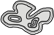
4 Fringe-Retrieving A*
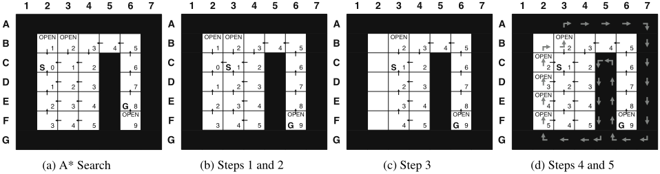
Fringe-Retrieving A* (FRA*) is an incremental version of A* that repeatedly transforms the previous search tree, which is given by the OPEN and CLOSED lists as well as the parents and g-values of the cells in them, to the current search tree, see the pseudo code in Figure 4. 2 Assume that FRA* finds a shortest path from the start cell, which is the current cell of the hunter, to the goal cell, which is the current cell of the target. Properties 1 and 2 hold afterwards since FRA* performs A* searches. Then, the hunter moves along the shortest path. When the target moves off the shortest path (that is, its current cell is not on the shortest path from the previous start cell to the previous goal cell any longer), FRA* changes the OPEN and CLOSED lists as well as the parents of the cells in them to guarantee that Properties 1 and 2 hold again and then starts an A* search with these OPEN and CLOSED lists to find a shortest path from the new start cell to the new goal cell. We use the four-neighbor gridworld in Figure 2 to illustrate the steps of FRA*. The current cell C2 of the hunter is labeled S, and the current cell E6 of the target is labeled G. Figure 2(a) shows the very first search of FRA*, which is an A* search from C2 to E6. Cells in the OPEN and CLOSED list are labeled with their g-values in their lower right corners. The outgoing arrows point to their parents. Cells in the OPEN list are labeled OPEN. The shortest path is C2, C3, C4, B4, B5, B6, C6, D6 and E6. The hunter then moves along the shortest path to C3, and the target moves off the shortest path to F6. FRA* now finds a shortest path from C3 to F6 using the following steps.
1 Figure 1 illustrates what we call the inner and outer perimeters of an area. The solid black line is the outer perimeter of the grey area, and the dashed black line is the inner perimeter of the grey area. The outer and inner perimeters consist of three parts each.
2 The following explanations are intended to make the pseudo code easier to understand: ComputeShortestPath() performs an A* search. iteration is the number of the current search. InitializeCell(s) initializes g(s) to infinity, generatediteration(s) to the number of the current search and expanded(s) to false when cell s is generated during a search. generatediteration(s) is set to the number of the current search when s is generated. expanded(s) is set to true when s is expanded. TestClosedList(s) returns true iff s is in the CLOSED list. It returns true iff s = sstart OR (expanded(s) AND parent(s) ̸= NULL). FRA* sometimes sets only expanded(s) to false and sometimes only parent(s) to NULL to delete s from the CLOSED list, which speeds it up.
4.1 Step 1: Starting A* Immediately
If the new start cell is the same as the previous start cell and the new goal cell is in the previous CLOSED list, then one can identify a shortest path from the new start cell to the new goal cell in reverse by following the existing parents from the new goal cell to the new start cell according to Property 1. If the new start cell is the same as the previous start cell and the new goal cell is not in the previous CLOSED list, then FRA* starts an A* search with the previous OPEN and CLOSED lists and does not need to execute the following steps. In our example, these conditions are not satisfied and FRA* thus executes the following steps.
4.2 Optional Step 2: Changing Parents
The new CLOSED list needs to satisfy Property 1 with respect to the new start cell. The previous CLOSED list satisfies Property 1 with respect to the previous start cell since FRA* performs A* searches. If the new CLOSED list contains exactly all cells of the subtree of the search tree rooted at the new start cell that are in the previous CLOSED list, then Property 1 holds with respect to the new start cell. Property 1(a) holds trivially, and Property 1(b) holds for the following reason: Consider the shortest path from the previous start cell s′start to any cell s in the new CLOSED list that results from following the parents from s to s′start in reverse. Since the the new start cell sstart is on this shortest path, it holds that d(s′start, s) = d(s′start, sstart) + d(sstart, s). Since cell s satisfies Property 1(b) with respect to the old start cell, it holds that g(s) = g(s′start) + d(s′start , s). Since cell sstart satisfies Property 1(b) with respect to the old start cell, it holds that g(sstart) = g(s′start)+d(s′start, sstart). Thus, cell s also satisfies Property 1(b) with respect to the new start cell since g(s) = g(s′start)+d(s′start, s) = g(sstart)-d(s′start , sstart)+d(s′start , s) = g(sstart)+d(sstart, s). However, the new CLOSED list should be as large a subset of the previous CLOSED list as possible. Cells from the previous CLOSED list often satisfy Property 1(b) with respect to the new start cell but not Property 1(a) since there are typically many alternative shortest paths from the previous start cell to a cell s in the previous CLOSED list. If the new start cell is on the shortest path from the previous start cell to s that results from following the parents from s to the previous start cell, then s is in the subtree of the search tree rooted at the new start cell and thus in the new CLOSED list. If the new start cell is not on the shortest path, then s is not in the subtree of the search tree rooted at the new start cell. FRA* finds such cells and changes their parents to make them part of the search tree rooted at the new start cell so that they can be part of the new CLOSED list. First, FRA* makes the new start cell its current cell, faces its parent and performs checks in the counter-clockwise direction. It turns counter-clockwise to face the next neighbor cell s′ of its current cell s that is in the previous CLOSED list and checks whether it holds that g(s′ ) = g(s) + c(s, s′ ).
- If the check is successful, then FRA* sets the parent of s′ to s, which is possible because this change does not affect its g-value. Due to this change, all cells in the subtree of the search tree rooted at s′ now belong to the subtree of the search tree rooted at the new start cell and their g-values remain unaffected. FRA* then makes s′ its current cell, faces its new parent s and repeats the
- process of turning and checking the neighbor cell that it faces.
- If the check is unsuccessful, then FRA* repeats the process of turning and checking the neighbor cell that it faces.
If, during the process of turning and checking the neighbor cell that it faces, FSA* faces the parent of its current cell again, then it makes the new start cell its current cell again, faces its parent and now performs similar checks in the clockwise direction. The resulting search tree is one that an A* search could have generated if it had broken ties among cells with the same sum of g-value and h-value appropriately. Step 2 traverses at most the inner perimeter of the new CLOSED list, which can be expected to contain fewer cells than the CLOSED list itself.
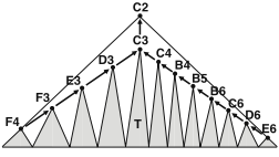
In our example, the cells in the subtree of the search tree rooted at the new start cell C3 before Step 2 that are in the previous CLOSED list are B4, B5, B6, C3, C4, C6, D6 and E6. However, D3 could have C3 as parent rather than D2 since this change does not affect its g-value. Then, all cells in the subtree of the search tree rooted at D3 belong to this subtree and their g-values remain unaffected. FRA* starts at the new start cell C3 and performs checks in the counter-clockwise direction. First, FRA* is at C3 facing its parent C2 and checks D3 successfully. It then sets the parent of D3 to C3. Second, FRA* is at D3 facing its parent C3, checks D2 unsuccessfully and then checks E3 successfully. It then sets the parent of E3 to D3. Third, FRA* is at E3 facing its parent D3, checks E2 unsuccessfully and then checks F3 successfully. It then sets the parent of F3 to E3. Fourth, FRA* is at F3 facing its parent E3, checks F2 unsuccessfully and then checks F4 successfully. It then sets the parent of F4 to F3 (which does not change its parent). Fifth, FRA* is at F4 facing its parent F3 and checks E4 unsuccessfully. FRA* then starts again at the new start cell C3 and performs similar checks in the clockwise direction until it reaches E6, see Figure 2(b). The cells in the subtree of the search tree rooted at the new start cell C3 after Step 2 that are in the previous CLOSED list are B4, B5, B6, C3, C4, C6, D3, D4, D6, E3, E4, E6, F3, F4 and F6. The big triangle in the conceptual Figure 3 represents all cells in the search tree that are in the previous CLOSED list, the triangle T in the big triangle represents all cells in the subtree of the search tree rooted at the new start cell before Step 2 that are in the previous CLOSED list, and the area in the big triangle below and including the cells traversed by FRA* in the counter-clockwise direction (C3, D3, E3, F3 and F4) and the clockwise direction (C3, C4, B4, B5, B6, C6, D6, and E6) represents all cells in the subtree of the search tree rooted at the new start cell after Step 2 that are in the previous CLOSED list.
4.3 Step 3: Deleting Cells
FRA* now generates the new CLOSED list, which contains exactly all cells of the subtree of the search tree rooted at the new start cell that are in the previous CLOSED list. Thus, FRA* could set the new CLOSED list to empty and then use breadth-first or depth-first search to traverse this subtree, starting with the new start cell, and insert the visited cells that
procedure InitializeCell(s) {01} if (generatediteration(s) ̸= iteration) {02} g(s) :=∞; {03} generatediteration(s) := iteration; {04} expanded(s) := false; function TestClosedList(s) {05} return (s = sstart OR (expanded(s) AND parent(s) ̸= NULL)); function ComputeShortestPath() {06} while (OPEN ̸= ∅) {07} delete a state s with the smallest g(s) +h(s, sgoal) fromOPEN; {08} expanded(s) := true; {09} forall s′ ∈ N(s) {10} if (NOT TestClosedList(s′ )) {11} InitializeCell(s′ ); {12} if (g(s′ ) > g(s) + c(s, s′ )) {13} g(s′ ) := g(s) + c(s, s′ ); {14} parent(s′ ) := s; {15} insert s′ into OPEN if s′ is not in OPEN; {16} return true if (s = sgoal ); {17} return false; function UpdateParent(direction) {18} forall s ∈ N(cell) in direction order, starting with parent(cell) {19} if (g(s) = g(cell) + c(cell, s) AND TestClosedList(s)) {20} parent(s) := cell; {21} cell := s; {22} return true; {23} return false; procedure Step2() {24} cell := sstart ; {25} while (UpdateParent(counter-clockwise)) /* body of while-loop is empty */; {26} cell := sstart ; {27} while (UpdateParent(clockwise)) /* body of while-loop is empty */; function Step3() {28} parent(sstart) := NULL; {29} forall s ∈ S that belong to the search tree rooted at previous sstart {30} parent(s) := NULL; {31} delete s fromOPEN if s ∈ OPEN; procedure Step5() {32} forall s ∈ S on the outer perimeter of the CLOSED list, starting with anchor a {33} OPEN := OPEN∪ {s} if (s is unblocked AND s /∈ OPEN); {34} forall s ∈ OPEN {35} InitializeCell(s); {36} forall s ∈ OPEN {37} forall s′ ∈ N(s) {38} if (TestClosedList(s′ ) AND g(s) > g(s′ ) + c(s′ , s)) {39} g(s) := g(s′ ) + c(s′ , s); {40} parent(s) := s′ ; {41} insert s into OPEN if s is not in OPEN; function Main() {42} forall s ∈ S {43} generatediteration(s) := 0; {44} expanded(s) := false; {45} iteration := 1; {46} InitializeCell(sstart); {47} g(sstart) := 0; {48} OPEN := ∅; {49} insert sstart into OPEN; {50} while (sstart ̸= sgoal ) {51} return false if (NOT ComputeShortestPath()); {52} openlist incomplete := false; {53} while (TestClosedList(sgoal)) /* Check of Steps 1 and 4 */ {54} while (target not caught and target is on shortest path from sstart to sgoal) {55} follow shortest path from sstart to sgoal; {56} return true if target caught; {57} previous sstart := sstart ; {58} sstart := the current cell of the hunter; {59} sgoal := the current cell of the target; {60} if (sstart ̸= previous sstart) /* Check of Step 1 */ {61} Step2(); {62} anchor := parent(sstart); {63} Step3(); {64} openlist incomplete := true; {65} if (openlist incomplete) {66} iteration := iteration + 1; {67} Step5(); {68} return true;a The CLOSED list contains exactly all cells s′ ∈ S with TestClosedList(s′). The forall-loop iterates only over the cells on the part of the outer perimeter of the CLOSED list that contains the anchor cell anchor.
Figure 4: Fringe Retrieving A* (FRA*).
are in the previous CLOSED list into the new CLOSED list to form the new CLOSED list. However, FRA* can also do the opposite. It can use breadth-first or depth-first search to traverse the search tree except for the subtree rooted at the new start cell, starting with the previous start cell, and delete the visited cells that are in the previous CLOSED list from the previous CLOSED list to form the new CLOSED list. The second option is usually faster since the hunter typically cannot move far along the shortest path before the target moves off the path. Thus, the previous and new start cells are typically much closer to each other than the new start and goal cells, meaning that there are only few cells to delete from the previous CLOSED list. Therefore, FRA* remembers the parent of the new start cell (that we call the anchor cell). It then sets the parent of the new start cell to NULL to disconnect this subtree from the search tree and uses breadth-first search to traverse the resulting search tree, starting with the previous start cell, and deletes the visited cells that are in the previous CLOSED list from the previous CLOSED list to form the new CLOSED list. It also deletes the visited cells that are not in the previous CLOSED list from the previous OPEN list to form the new OPEN list. Afterwards, the new CLOSED list is complete. The parents and g-values of all cells in the new CLOSED list satisfy Property 1.
In our example, FRA* sets the parent of C2 to NULL, it then deletes C2, D2, E2 and F2 from the previous CLOSED list and deletes B2 from the previous OPEN list, see Figure 2(c).
4.4 Step 4: Terminating Early
If the new goal cell is in the new CLOSED list then one can identify a shortest path from the new start cell to the new goal cell in reverse by following the parents from the new goal cell to the new start cell according to Property 1. In our example, this condition is not satisfied and FRA* thus executes the following steps.
4.5 Step 5: Inserting Cells
The new OPEN list needs to contain exactly all cells that are on the outer perimeter of the CLOSED list according to Property 2. The cells that are on the part of the outer perimeter of the CLOSED list that does not contain the anchor cell from Step 3 are already in the new OPEN list. However, not all cells on the part of the outer perimeter of the CLOSED list that contains the anchor cell are necessarily already in the new OPEN list. In particular, it could be the case that some of the cells that were in the previous CLOSED list but are not in the new CLOSED list should now be in the OPEN list. The new CLOSED list forms a contiguous area according to Property 1. FRA* thus completes the new OPEN list by circumnavigating the part of the outer perimeter of the new CLOSED list that contains the anchor cell, starting with the anchor cell, and inserting every visited unblocked cell that is not yet in the new OPEN list into the new OPEN list. Afterwards, the new OPEN list is complete. However, the parents and g-values of some cells in the new OPEN list might not satisfy Property 2. FRA* therefore sets the parent of every cell s in the newOPEN list to the cell s′ in the new CLOSED list that minimizes g(s′ )+c(s′ , s) and then the g-value of s to g(parent(s)) + c(parent(s), s). The parents and g-values of all cells in the new OPEN list now satisfy Property 2. Step 5, different from [Edelkamp, 1998], traverses at most the outer perimeter of the new CLOSED list, which can be expected to contain fewer cells than the CLOSED list itself.
| Four-Neighbor Maze | ||||||
|---|---|---|---|---|---|---|
| searches per test case | moves per test case | cells expanded per search | cells removed fromCLOSED per search | total runtime per search | ||
| A* | 4218 | 6716 | 174127 (212) | 45388 | ||
| MT-Adaptive A* | 4218 | 6716 | 94362 (131) | 35268 | ||
| Differential A* | 4218 | 6716 | 174127 (212) | 63008 | ||
| Basic FRA* | 4242 | 6712 | 472 (3.8) | 522 | (6.5) | 674 |
| FRA* | 4242 | 6712 | 461 (3.7) | 502 | (6.2) | 655 |
In our example, FRA* circumnavigates the part of the outer perimeter of the new CLOSED list that contains C2, starting with C2, and inserts C2, D2, E2 and F2 into the previous OPEN list and then corrects all of their parents and g-values. For example, the parent of D2 was C2 and its g-value was one. FRA* sets the parent of D2 to D3 and its g-value to three, see Figure 2(d).
4.6 Step 6: Starting A*
FRA* starts an A* search with the new OPEN and CLOSED lists. The g-value of the new start cell is not necessarily zero at this point in time since FRA* has not changed it since its previous search.
5 Experimental Evaluation
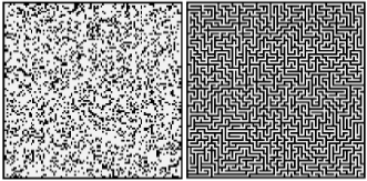
We compare Basic FRA* (without the optional Step 2) and FRA* (with the optional Step 2) experimentally against A*, MT-Adaptive A* (which is identical to Generalized MTAdaptive A* in known gridworlds), Differential A* and D* Lite (which is simpler than D* but as efficient [Koenig and Likhachev, 2005]). We use comparable implementations for all search algorithms. For example, all of them use binary heaps as priority queues. We use four-neighbor and eightneighbor random gridworlds in which 25 percent of randomly chosen cells were blocked and four-neighbor mazes whose corridors and walls are ten cells wide and whose corridors were generated with depth-first search, see Figure 5. We average over 1000 gridworlds of size 1000 × 1000 whose start and goal cells were randomly chosen. The target always follows a shortest path from its current cell to a randomly selected unblocked cell and repeats the process once it reaches that cell. The target skips every tenth move, which enables the hunter to catch it.
Tables 1 and 2 report two measures for the difficulty of the moving target search problems (that vary slightly among moving target search algorithms due to different tie breaking among several shortest paths), namely the average number of searches and the average number of moves of the hunter until it catches the target. The tables report two measures for the efficiency of the moving target search algorithms, namely the average number of expanded cells per search and the average runtime per search in microseconds on a Pentium D 3.0 Ghz PC with 2 GByte of RAM. The tables also report the average number of cells per search that Basic FRA* and FRA* remove from the CLOSED list. Finally, the tables report the standard deviation of the mean for the number of expanded cells per search and the number of cells removed from the CLOSED list per search (in parentheses) to demonstrate the statistical significance of our results. D* Lite is not listed in the table because it exceeds our runtime limit of 10 hours for the 1000 gridworlds that we average over and is thus not competitive.
| Four-Neighbor Random Gridworld | Eight-Neighbor Random Gridworld | ||||||||||||
|---|---|---|---|---|---|---|---|---|---|---|---|---|---|
| searches per test case | moves per test case | cells expanded per search | cells removed fromCLOSED per search | total runtime per search | searches per test case | moves per test case | cells expanded per search | cells removed fromCLOSED per search | total runtime per search | ||||
| A* | 387 | 688 | 14013 | (31.2) | 7250 | 335 | 475 | 8418 | (19.3) | 6098 | |||
| MT-Adaptive A* | 387 | 688 | 12351 | (28.2) | 6002 | 335 | 475 | 8001 | (21.9) | 6078 | |||
| Differential A* | 387 | 688 | 14013 | (40.1) | 9533 | 335 | 475 | 8418 | (19.3) | 7355 | |||
| Basic FRA* | 391 | 688 | 541 | (13.1) | 386 (12.3) | 422 | 336 | 477 | 350 | (3.9) | 276 | (8.1) | 464 |
| FRA* | 391 | 688 | 515 | (13.0) | 362 (11.6) | 397 | 336 | 477 | 325 | (3.8) | 256 | (7.5) | 438 |
In all cases, the sum of the average number of cells that Basic FRA* expands and the average number of cells that it removes from the CLOSED list is an order of magnitude smaller than the average number of cells that the other search algorithms expand. Accordingly, the average runtime of Basic FRA* is an order of magnitude smaller than the average runtime of the other search algorithms. FRA* is even faster than Basic FRA*, which demonstrates the utility of the optional Step 2.
6 Conclusions
In this paper, we developed Fringe-Retrieving A* (FRA*), an incremental search algorithm that repeatedly finds shortest paths for moving target search in known gridworlds. We demonstrated experimentally that it runs up to one order of magnitude faster than a variety of state-of-the-art incremental search algorithms applied to moving target search in known gridworlds, namely D* Lite, Differential A* and MT-Adaptive A*. FRA* is faster than the other incremental search algorithms because moving target search poses a problem for them. None of the other incremental search algorithms that transform the previous search tree to the current search tree were specifically designed for moving target search. They are efficient only if the start cell remains unchanged from search to search. Thus, they are not efficient for moving target search, where both the start and goal cells change over time. For example, D* Lite needs to shift the map and cannot reuse much of the previous search tree [Koenig et al., 2007], and Differential A* cannot reuse the previous search tree at all, which makes both of them slower than A*. MT-Adaptive A* is an incremental search algorithm that uses information from the previous searches to update the h-values of the current search. It was specifically designed for moving target search but does not transform the previous search tree to the current search tree. FRA* is thus the first incremental search algorithm that efficiently transforms the previous search tree to the current search tree for moving target search in known gridworlds.
@inproceedings{ijcai2009p108,
  title     = {Efficient Incremental Search for Moving Target Search},
  author    = {Sun, Xiaoxun and Yeoh, William and Koenig, Sven},
  booktitle = {Proceedings of the Twenty-First International Joint Conference on
               Artificial Intelligence, {IJCAI-09}},
  publisher = {International Joint Conferences on Artificial Intelligence},
  editor    = {Craig Boutilier},
  pages     = {615--619},
  year      = {2009},
  url       = {https://ijcai.org/proceedings/2009/108},
}
TY - CPAPER TI - Efficient Incremental Search for Moving Target Search AU - Sun, Xiaoxun AU - Yeoh, William AU - Koenig, Sven T2 - Proceedings of the Twenty-First International Joint Conference on Artificial Intelligence, IJCAI-09 PB - International Joint Conferences on Artificial Intelligence PY - 2009 SP - 615 EP - 619 UR - https://ijcai.org/proceedings/2009/108 ER -Copied
Machine-readable versions of this paper, for tools and AI agents:





