
The Focussed D* Algorithm for Real-Time Replanning
Proceedings of the Fourteenth International Joint Conference on Artificial Intelligence. Planning. Pages 1662-1668.
© 1995 International Joint Conferences on Artificial Intelligence
Abstract
Finding the lowest-cost path through a graph is central to many problems, including route planning for a mobile robot. If arc costs change during the traverse, then the remainder of the path may need to be replanned. Tbis is the case for a sensor-equipped mobile robot with imperfect information about its environment. As the robot acquires additional information via its sensors, it can revise its plan to reduce the total cost of the traverse. If the prior information is grossly incomplete, the robot may discover useful information in every piece of sensor data. During replanning, the robot must either wait for the new path to be computed or move in the wrong direction; therefore, rapid replanning is essential. The D* algorithm (Dynamic A*) plans optimal traverses in real-time by incrementally repairing paths to the robot's state as new information is discovered. This paper describes an extension to D* that focusses the repairs to significantly reduce the total time required for the initial path calculation and subsequent replanning operations. This extension completes the development of the D* algorithm as a full generalization of A* for dynamic environments, where arc costs can change during the traverse of the solution path.
- [Boult, 1987] T. Boult. Updating distance maps when objects move. In Proceedings of the SPIE Conference on Mobile Robots, 1987.
- [Jarvis, 1985] R. A. Jarvis. Collision-free trajectory plan- ning using the distance transforms. Mechanical Engineering Trans. of the Institution of Engineers, M£10(3), September 1985.
- [Korf, 1987] R. E . Korf. Real-time heuristic search: first results. In Proceedings of the Sixth National Conference on Artificial Intelligence, July 1987.
- [Lumelsky and Stepanov, 1986] V. J. Lumelsky and A. A. Stepanov. Dynamic path planning for a mobile automaton with limited information on the environment. IEEE Transac- tions on Automatic Control, AC-31(11), November 1986.
- [Nilsson, 1980] N.J. Nilsson. Principles of Artificial Intelli- gence, Tioga Publishing Company, 1980, pp. 72-88.
- [Pirzadeh and Snyder, 1990] A. Pirzadeh and W. Snyder. A unified solution to coverage and search in explored and unexplored terrains using indirect control. In Proceedings of the IEEE International Conference on Robotics and Automa- tion, May 1990.
- [Ramalingam and Reps, 1992] G. Ramalingam and T. Reps. An incremental algorithm for a generalization of the short- est-path problem. University of Wisconsin Technical Report #1087, May 1992.
- [Stentz, 1993] A. Stentz. Optimal and efficient path plan- ning for unknown and dynamic environments. Carnegie Mellon Robotics Institute Technical Report CMU-RI-TR- 93-20, August 1993.
- [Stentz, 1994] A. Stentz. Optimal and efficient path plan- ning for partially-known environments. In Proceedings of the IEEE International Conference on Robotics and Automa- tion, May 1994.
- [Trovato, 1990] K. I. Trovato. Differential A*: an adaptive search method illustrated with robot path planning for mov- ing obstacles and goals, and an uncertain environment. Jour- nal of Pattern Recognition and Artificial Intelligence, 4(2), 1990.
- [Zelinsky, 1992] A. Zelinsky. A mobile robot exploration algorithm. IEEE Transactions on Robotics and Automation, 8(6), December 1992.
References were extracted automatically from the PDF and may contain errors.
Full text extracted automatically from the PDF; figures, tables and equations may differ. The PDF is the version of record.
1 Introduction
The problem of path planning can be stated as finding a sequence of state transitions through a graph from some ini tial state to a goal state, or determining that no such sequence exists. The path is optimal if the sum of the transition costs, also called arc costs, is minimal across all possible sequences through the graph. If during the "traverse" of the path, one or more arc costs in the graph is discovered to be these limitations with D*, an incremental algorithm which maintains a partial, optimal cost map limited to those locations likely to be of use to the robot. Likewise, repair of the cost map is generally partial and re-entrant, thus reducing computational costs and enabling real-time performance.
1. This research was sponsored by ARPA, under contracts "Per ception for Outdoor Navigation" (contract number DACA76-89-C0014, monitored by the US Army TEC) and "Unmanned Ground Vehicle System" (contract number DAAE07-90-C-R059, moni tored by TACOM).
Other algorithms exist for addressing the problem of path planning in unknown or dynamic environments [Korf, 1987; Lumelsky and Stepanov, 1986; Pirzadeh and Snyder, 1990], but these algorithms emphasize fast operation and/or low memory usage at the expense of optimality.
This paper describes an extension to D* which focusses the cost updates to minimize state expansions and further reduce computational costs. The algorithm uses a heuristic function similar to A* to both propagate cost increases and focus cost reductions . A biasing function is used to compensate for robot motion between replanning operations. The net effect is a reduction in run-time by a factor of two to three. The paper begins with the intuition behind the algorithm, describes the extension, presents an example, evaluates empirical comparisons, and draws conclusions.
2 Intuition for Algorithm
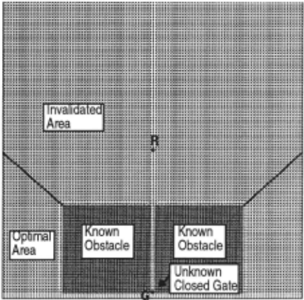
Consider how A* solves the following robot path planning problem. Figure 1 shows an eight-connected graph repre senting a Cartesian space of robot locations. The states in the graph, depicted by arrows, are robot locations, and the arcs encode the cost of moving between states. The white regions are locations known to be in free space. The arc cost for moving between free states is a small value denoted by EMPTY . The grey regions are known obstacle locations, and arcs connected to these states are assigned a prohibitively high value of OBSTACLE. The small black square is a closed gate believed to be open (i.e., EMPTY value). With out a loss of generality, the robot is assumed to be point-size and occupies only one location at a time. A* can be used to compute optimal path costs from the goal, G , to all states in the space given the initial set of arc costs, as shown in the figure. The arrows indicate the optimal state transitions; therefore, the optimal path for any state can be recovered by following the arrows to the goal. Because the closed gate is assumed to be open, A* plans a path through it.
The robot starts at some initial location and begins following the optimal path to the goal. At location R, the robot's sensor discovers the gate between the two large obstacles is closed. This corresponds to an incorrect arc value in the graph: rather than EMPTY, it has a much higher value of GATE, representing the cost of first opening the gate and then moving through it. All paths through this arc are (possibly) no longer optimal, as indicated by the labelled region. A* could be used to recompute the cost map, but this is inefficient if the environment is large and/or the goal is far away.
Several characteristics of the problem motivate a better approach. First, changes to the arc costs are likely to be in the vicinity of the robot, since it typically carries a sensor with a limited range. This means that most plans need only be patched "locally". Second, the robot generally makes near-monotonic progress toward the goal. Most obstructions are small and simple path deflections suffice, thus avoiding the high computational cost of backtracking. Third, only the remaining portion of the path must be replanned at a given location in the traverse, which tends to get progressively shorter due to the second characteristic.
As described in Stentz [1994] , D* leverages on these characteristics to reduce run-time by a factor of 200 or more for large environments. The paper proves that the algorithm produces correct results regardless--only the performance improvement is affected by the validity of the problem characteristics.
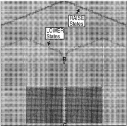
Like A*, D* maintains an OPEN list of states for expansion; however, these states consist of two types : RAISE and LOWER . RAISE states transmit path cost increases due to an increased arc value, and LOWER states reduce costs and re-direct arrows to compute new optimal paths. The RAISE states propagate the arc cost increase through the invalidated states, by starting at the gate and sweeping outward, adding the value of GATE to all states in the region. The RAISE states activate neighboring LOWER states which sweep in behind to reduce costs and re-direct pointers. LOWER states compute new, optimal paths to the states that were previously raised.
States are placed on the OPEN list by their key value, k(X), which for LOWER states is the current path cost, h(X) (i.e., cost from the state X to the goal), and for RAISE states the previous, unraised h(X) value. States on the list are processed in order of increasing key value. The intuition is that the previous optimal path costs of the RAISE states define a lower bound on the path costs of LOWER states they can discover. Thus, if the path costs of the LOWER states currently on the OPEN list exceed the previous path costs of the RAISE states, then it is worthwhile processing RAISE states to discover (possibly) a better LOWER state.
The process can terminate when the lowest value on the OPEN list equals or exceeds the robot's path cost, since additional expan~ions cannot possibly find a better path to the goal (see Figure 2) . Once a new optimal path is computed or the old one is determined to be valid, the robot can continue to move toward the goal. Note in the figure that only part of the cost map has been repaired. This is the efficiency of the D* algorithm.
The D* algorithm described in Stentz [1994] propagates cost changes through the invalidated states without considering which expansions will benefit the robot at its current location. Like A*, D* can use heuristics to focus the search in the direction of the robot and reduce the total number of state expansions. Let the focussing heuristic g(X, R) be the estimated path cost from the robot's location R to X. Define a new function, the estimated robot path cost, to be f(X, R) = h(X) + g(X, R), and sort all LOWER states on the OPEN list by increasing ft 0 ) value. The function f(X, R) is the estimated path cost from the state R through X to G . Provided that g( 0 ) satisfies the monotone restriction, then since h(X) is optimal when LOWER state X is removed from the OPEN list, an optimal path will be computed to R [Nilsson, 1980] . The notation g( 0 ) is used to refer to a function independent of its domain.
In the case of RAISE states, the previous h( 0 ) value defines a lower bound on the h( 0 ) values of LOWER states they can discover; therefore, if the same focussing heuristic g( 0 ) is used for both types of states, the previous j( 0 ) values of the RAISE states define lower bounds on the ft 0 ) values of the LOWER states they can discover. Thus, if the [( 0 ) values of the LOWER states on the OPEN list exceed the previous [( 0 ) values of the RAISE states, then it is worthwhile processing RAISE states to discover better LOWER states. Based on this reasoning, the RAISE states should be sorted on the OPEN list by f(X,R) = k(X)+g(X,R) . But since k(X) = h(X) for LOWER states, the RAISE state definition for {( 0 ) suffices for both kinds of states. To avoid cycles in the backpointers, it should be noted that ties in ft 0 ) are sorted by increasing k( 0 ) on the OPEN list [Stentz, 1993] .
The process can terminate when the lowest value on the OPEN list equals or exceeds the robot's path cost, since the subsequent expansions cannot possibly find a LOWER state that 1) has a low enough path cost, and 2) is "close" enough to the robot to be able to reduce the robot's path cost when it reaches it through subsequent expansions. Note that this is a more efficient cut-off than the previous one, which considers only the first criterion.
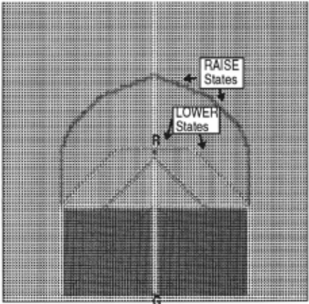
Figure 3 shows the same example, except that a focussed search is used. All states in the RAISE state wave front have roughly the same ft 0 ) value. The wave front is more "narrow" in the focussed case since the inclusion of the cost to return to the robot penalizes the wide flanks. Furthermore, the LOWER states activated by the RAISE state wave front have swept in from the outer sides of the obstacles to compute a new, optimal path to the robot. Note that the two wave fronts are narrow and focussed on the robot's location. Compare Figure 3 to Figure 2. Note that both the RAISE and LOWER state wave fronts have covered less ground for the focussed search than the unfocussed search in order to compute a new, optimal path to R . Therein is the efficiency of the Focussed D* algorithm.
The problem with focussing the search is that once a new optimal path is computed to the robot's location, the robot then moves to a new location. If its sensor discovers another arc cost discrepancy, the search should be focussed on the robot's new location. But states already on the OPEN list are focussed on the old location and have incorrect g( 0 ) and ft 0 ) values. One solution is to recompute g( 0 ) and f{') for all states on the OPEN list every time the robot moves and new states are to be added. Based on empirical evidence, the cost of re-sorting the OPEN list more than offsets the savings gained by a focussed search.
The approach in this paper is to take advantage of the fact that the robot generally moves only a few states between replanning operations, so the g( 0 ) and f{ 0 ) values have only a small amount of error. Assume that state X is placed on the OPEN list when the robot is at location R 0 · Its f{ 0 ) value at that point is ftX, R 0 ). If the robot moves to location R 1 , we could calculate ftX, R 1 ) and adjust its position on the OPEN list. To avoid this computational cost, we compute a lower bound on f(X, R 1 ) given by fL(X, R 1 ) = f(X, R 0 ) - g(RI' R 0 ) - E. h<X. R 1 ) is a lower bound on f(X, R 1 ) since it assumes the robot moved in the "direction" of state X, thus subtracting the motion from g(X, R 0 ) . The parameter E is an arbitrarily small positive number. If X is repositioned on the OPEN list by h(X,R 1 ), then since h(X, R 1 ) is a lower bound on f(X, R 1 ), X will be selected for expansion before or when it is needed. At the time of expansion, the true f(X, R 1 ) value is computed, and X is placed back on the OPEN list by f(X, R 1 ).
At first this approach appears worse, since the oPEN list is first re-sorted by h( 0 ) and then partially adjusted to replace the h( 0 ) values with the correct {( 0 ) values. But since g(R I' R 0 ) + E is subtracted from all states on the oPEN list, the ordering is preserved, and the list need not be re-sorted. Furthermore, the first step can be avoided altogether by adding g(RI' R 0 ) + E to the states to be inserted on the OPEN list rather than subtracting it from those already on the list, thus preserving the relative ordering between states already on the list and states about to be added. Therefore, the only remaining computation is the adjustment step. But this step is needed only for those states that show promise for reaching the robot's location. For typical problems, this amounts to fewer than 2% of the states on the OPEN list.
3 Definitions and Formulation
To formalize this intuition, we begin with the notation and definitions used in Stentz [1994], and then extend it for the focussed algorithm. The problem space can be formulated as a set of states denoting robot locations connected by direc tional arcs, each of which has an associated cost. The robot starts at a particular state and moves across arcs (incurring the cost of traversal) to other states until it reaches the goal state, denoted by G . Every visited state X except G has a backpointer to a next state Y denoted by b(X) = Y . D* uses backpointers to represent paths to the goal. The cost of tra versing an arc from state Y to state X is a positive number given by the arc cost function c(X, Y) . If Y does not have an arc to X, then c(X, Y) is undefined. Two states X and Y are neighbors in the space if c(X, Y) or c(Y, X) is defined.
D* uses an OPEN list to propagate information about changes to the arc cost function and to calculate path costs to states in the space. Every state X has an associated tag t(X) , such that t(X) = NEW if X has never been on the OPEN list, t(X) = OPEN if X is currently on the OPEN list, and t(X) = CLOSED if X is no longer on the OPEN list. For each visited state X, D* maintains an estimate of the sum of the arc costs from X to G given by the path cost function h(X) . Given the proper conditions, this estimate is equivalent to the optimal (minimal) cost from state X to G. For each state X on the OPEN list (i.e., t(X) = OPEN), the key function, k(X) ; is defined to be equal to the minimum of h(X) before modification and all values assumed by h(X) since X was placed on the OPEN list. The key function classifies a state X on the OPEN list into one of two types: a RAISE state if k(X) < h(X), and a LOWER state if k(X) = h(X). D* uses RAISE states on the OPEN list to propagate information about path cost increases and LOWER states to propagate information about path cost reductions. The propagation takes place through the repeated removal of states from the OPEN list. Each time a state is removed from the list, it is expanded to pass cost changes to its neighbors.
These neighbors are in turn placed on the OPEN list to continue the process.
States are sorted on the OPEN list by a biased {( 0 ) value, given by f 8 (X, Ri), where X is the state on the OPEN list and Ri is the robot's state at the time X was inserted or adjusted on the OPEN list. Let {R 0 , Rl' ... , RN} be the sequence of states occupied by the robot when states were added to the OPEN list. The value of { 8 ( 0 ) is given by { 8 (X, R;) = f(X, R;) + d(Ri, R 0 ), where {( 0 ) is the estimated robot path cost given by f(X, Ri) = h(X) + g(X, Ri) and d( 0 ) is the accrued bias function given by d(Ri, R 0 ) = g(R I' R 0 ) + g(R 2 , R 1 ) + ... + g(Ri, Ri _ 1 ) + iE if i > o and d(R 0 , R 0 ) = o if i = o . The function g(X, Y) is the focussing heuristic, representing the estimated path cost from Y to X. The OPEN list states are sorted by increasing { 8 ( 0 ) value, with ties in { 8 ( 0 ) ordered by increasing {( 0 ) , and ties in 1( 0 ) ordered by increasing W). Ties in W) are ordered arbitrarily. Thus, a vector of values (! 8 ( 0 ),/( 0 ) , W)) is stored with each state on the list.
Whenever a state is removed from the OPEN list, its 1( 0 ) value is examined to see if it was computed using the most recent focal point. If not, its tn and { 8 ( 0 ) values are recalculated using the new focal point and accrued bias, respectively, and the state is placed back on the list. Processing the t 8 ca> values in ascending order ensures that the first encountered {( 0 ) value using the current focal point is the minimum such value, denoted by fmin . Let kval be its corresponding k( 0 ) value. These parameters comprise an important threshold forD*. By processing properly-focussed 1( 0 ) values in ascending order (and kCO) values in ascending order for a constant 1( 0 ) value), the algorithm ensures that for all states X, if /{X) <!min or (/{X) = !min and h(X) ~ kval ), then h(X) is optimal. The parameter val is used to store the vector (!min' kvaz> for the purpose of this test.
Let Rcurr be the current state on which the search is focussed, initialized to the robot's start state. Define the robot state function r(X), which returns the robot's state when X was last inserted or adjusted on the OPEN list. The parameter dcurr is the accrued bias from the robot's start state to its current state; it is shorthand for d(Rcurr' R 0 ) and is initialized to dcurr = d(R 0 , R 0 ) = 0. The following shorthand notation is used for fa( 0 ) and {( 0 ): f 8 (X)=-f 8 (X, r(X)) andf{X)=-f{X, r(X)).
4 Algorithm Description
The D* algorithm consists primarily of three functions: PROCESS - STATE, MODIFY - COST, and MOVE - ROBOT. PROCESS - STATE computes optimal path costs to the goal, MODIFY - COST changes the arc cost function c( 0 ) and enters affected states on the 0 PEN list, and MOVE - ROBOT uses the two functions to move the robot optimally. The algorithms for PROCESS - STATE, MODIFY - COST, and MOVE - ROBOT are presented below along with three of the more detailed functions for managing the OPEN list: INSERT, MIN - STATE, and MIN - VAL . The user provides the function GVAL(X, Y) , which computes and returns the focussing heuristic g(X, Y) .
The embedded routines are: MIN( a, b) returns the minimum of the two scalar values a and b; LESS( a, b) takes a vector of values (a 1 , a 2 ) for a and a vector (bl' b 2 ) for b and returns TRUE if a 1 <b 1 or (a 1 = b 1 and a 2 <b 2 ); LESSEQ(a, b) takes two vectors a and b and returns TRUE if a 1 < b 1 or (a 1 = b 1 and a 2 ~ b 2 ); COST(X) computes f(X, Rcurr) = h(X) + GVAL(X, Rcurr) and returns the vector of values (/(X, Rcurr), h(X)) for a state X; DELETE(X) deletes state X from the OPEN list and sets t(X) = CLOSED; PUT - STATE(X) sets t(X) = OPEN and inserts X on the OPEN list according to the vector (JB(X),f(X), k(X)); and GET - STATE returns the state on the OPEN list with minimum vector value (NULL if the list is empty).
The INSERT function, given below, changes the value of h(X) to hnew and inserts or repositions X on the OPEN list. The value for k(X) is determined at lines L1 through LS. The remaining two values in the vector are computed at line L 7, and the state is inserted at line L8.
Function: INSERT (X, huew)
L1 if t(X) = NEW then k(X) = hnew L2 else L3 if t(X) = OPEN then lA k(X) = MIN(k(X), hnew); DELETE(X) LS else k(X) = MIN(h(X), hnew) L6 h(X) = hnew; r(X) = Rcurr L7 f(X) = k(X) + GVAL(X, Rcurr); /B(X) = f(X) + dcurr L8 PUT - STATE(X)The function MIN - STATE, given below, returns the state on the oPEN list with minimum W) value. In order to do this, the function retrieves the state on the oPEN list with lowest fB( 0 ) value. If the state was placed on the OPEN list when the robot was at a previous location (line L2), then it is re-inserted on the OPEN list at lines L3 and L4. This operation has the effect of correcting the state's accrued bias using the robot's current state while leaving the state's h( 0 ) and k( 0 ) values unchanged. MIN- STATE continues to retrieve states from the OPEN list until it finds one that was placed on the oPEN list with the robot at its current state.
Function: MIN-STATE()
L1 while X= GET - STATE( )"#NULL L2 if r(X) "# Rcurr then L3 hnew = h(X); h(X) = k(X) L4 DELETE(X); INSERT(X, hnew) LS else return X- L6 return NULL
The MIN - VAL function, given below, returns the {( 0 ) and W) values of the state on the OPEN list with minimum {( 0 ) value, that is, (fmin' kval> .
Function: MIN-VAL 0
L1 X= MIN - STATE( ) L2 if X= NULL then return NO - VAL L3 else return (f(X), k(X))In function PROCESS - STATE cost changes are propagated and new paths are computed. At lines L1 through L3, the state X with the lowest f( 0 ) value is removed from the OPEN list. If X is a LOWER state (i.e., k(X) = h(X)), its path cost is optimal. At lines L9 through L14, each neighbor Y of X is examined to see if its path cost can be lowered. Additionally, neighbor states that are NEW receive an initial path cost value, and cost changes are propagated to each neighbor Y that has a backpointer to X, regardless of whether the new cost is greater than or less than the old. Since these states are descendants of X, any change to the path cost of X affects their path costs as well. The backpointer of Y is redirected, if needed. All neighbors that receive a new path cost are placed on the 0 PEN list, so that they will propagate the cost changes to thei.i' neighbors.
Function: PROCESS-STATE ()
L1 X= MIN -STATE( ) L2 if X = NULL then return NO - VAL L3 val = (j(X), k(X)); kval = k(X); DELETE(X) lA if kval < h(X) then LS for each neighbor Y of X: L6 if t(Y) "#NEW and LESSEQ(COST(Y), val) and L7 h(X) > h(Y) + c(Y, X) then L8 b(X) = Y; h(X) = h(Y) + c(Y, X) L9 if kval = h(X) then LIO for each neighbor Y of X: Lll if t(Y) = NEW or L12 (b(Y) = X and h(Y) "# h(X) + c(X, Y)) or L13 ( b( Y) "# X and h( Y) > h(X) + c(X, Y)) then L14 b(Y) = X; INSERT(Y, h(X) + c(X, Y)) LIS else Ll6 for each neighbor Y of X: Ll7 if t(Y) = NEW or L18 (b(Y) = X and h(Y) "# h(X) + c(X, Y)) then L19 b(Y) = X; INSERT(Y, h(X) + c(X, Y)) L20 else L21 if b(Y) "#X and h( Y) > h(X) + c(X, Y) and L22 t(X) = CLOSED then L23 INSERT(X, h(X)) L24 else L25 if b( Y) "# X and h(X) > h( Y) + c( Y, X) and L26 t(Y) = CLOSED and L27 LESS(val, COST(Y)) then L28 INSERT(Y, h(Y)) L29 return MIN - VAL( )If X is a RAISE state, its path cost may not be optimal. Before X propagates cost changes to its neighbors, its optimal neighbors are examined at lines L4 through L8 to see if h(X) can be reduced. At lines L16 through L19, cost changes are propagated to NEW states and immediate descendants in the same way as for LOWER states. If X is able to lower the path cost of a state that is not an immediate descendant (lines L21 through L23), X is placed back on the OPEN list for future expansion. This action is required to avoid creating a closed loop in the backpointers [Stentz, 1993]. If the path cost of X is able to be reduced by a suboptimal neighbor (lines L25 through L28), the neighbor is placed back on the OPEN list. Thus, the update is "postponed" until the neighbor has an optimal path cost.
In function MODIFY - COST, the arc cost function is updated with the changed value. Since the path cost for state Y will change, X is placed on the OPEN list. When X is expanded via PROCESS - STATE, it computes a new h(Y) = h(X) + c(X, Y) and places Y on the OPEN list. Additional state expansions propagate the cost to the descendants of Y .
Function: MODIFY-COST (X, Y, cval)
- L1 c(X, Y) = eva!
- L2 if t(X) = CLOSED then INSERT(X, h(X))
- L3 return MIN - VAL( )
The function MOVE - ROBOT illustrates how to use PROCESS - STATE and MODIFY - COST to move the robot from state s through the environment to G along an optimal traverse. At lines L 1 through L4 of MOVE - ROBOT, t( 0 ) is set to NEW for all states, the accrued bias and focal point are initialized, h(G) is set to zero, and G is placed on the OPEN list. PROCESS-STATE is called repeatedly at lines L6 and L 7 until either an initial path is computed to the robot's state (i.e., t(S) = CLOSED) or it is determined that no path exists (i.e., val = NO - VAL and t(S) = NEW). The robot then proceeds to follow the backpointers until it either reaches the goal or discovers a discrepancy (line L11) between the sensor measurement of an arc costs( 0 ) and the stored arc cost c( 0 ) (e.g., due to a detected obstacle). Note that these discrepancies may occur anywhere, not just on the path to the goal. If the robot moved since the last time discrepancies were discovered, then its state R is saved as the new focal point, and the accrued bias, dcurr, is updated (lines Ll2 and Ll3). MODIFY- COST is called to correct c( 0 ) and place affected states on the OPEN list at line Ll5. PROCESS - STATE is then called repeatedly at line L17 to propagate costs and compute a new path to the goal. The robot continues to follow the backpointers toward the goal. The function returns GOAL-REACHED if the goal is found and NO- PATH if it is unreachable.
Function: MOVE-ROBOT (S, G)
L1 for each state X in the graph: L2 t(X) =NEW L3 L4 LS L6 L7 L8 L9 dcurr = O; Rcurr = S INSERT(G, 0) val = (0, 0) while t(S) "*CLOSED and val"* NO - VAL val = PROCESS - STATE( ) if t(S) = NEW then return NO - PATH R = S LlOwhile R* G: Lll if s(X, Y) * c(X, Y) for some (X,Y) then L12 if R *R then curr L13 dcurr = dcurr + GVAL(R, Rcurr) + E; Rcurr = R L14 for each (X,Y) such that s(X, Y) * c(X, Y): Ll5 val = MODIFY - COST(X, Y, s(X, Y)) L16 while LESS( val, COST(R)) and val"* NO - VAL Ll7 val= PROCESS - STATE() Ll8 R = b(R) Ll9return GOAL - REACHEDIt should be noted that line L8 in MOVE - ROBOT only detects the condition that no path exists from the robot's state to the goal if, for example, the graph is disconnected. It does not detect the condition that all paths to the goal are obstructed by obstacles. In order to provide for this capability, obstructed arcs can be assigned a large positive value of OBSTACLE and unobstructed arcs can be assigned a small positive value of EMPTY. OBSTACLE should be chosen such that it exceeds the longest possible path of EMPTY arcs in the graph. No unobstructed path exists to the goal from s if h(S) ~OBSTACLE after exiting the loop at line L6. Likewise, no unobstructed path exists to the goal from a stateR during the traverse if h(R) ~OBSTACLE after exiting the loop at line L16. Since R = Rcurr for a robot state R undergoing path recalculations, then g(R, R) = o and f(R, R) = h(R). Therefore, optimality is guaranteed for a stateR, if !min> h(R) or (!min = h(R) and kval ~ h(R) ).
5 Example
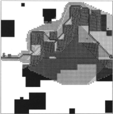
Figure 4 shows a cluttered 100 x 100 state environment. The robot starts at state s and moves to state G . All of the obsta cles, shown in black, are unknown before the robot starts its traverse, and the map contains only EMPTY arcs. The robot is point-size and is equipped with a 10-state radial field-of view sensor. The figure shows the robot's traverse from s to G using the Basic D* algorithm. The traverse is shown as a black curve with white arrows. As the robot moves, its sen sor detects the unknown obstacles. Detected obstacles are shown in grey with black arrows. Obstacles that remain unknown after the traverse are shown in solid black or black with white arrows. The arrows show the final cost field for all states examined during the traverse. Note that most of the states are examined at least once by the algorithm.
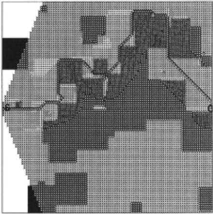
Figure 5 shows the robot's traverse using the Focussed D* algorithm. The number of NEW states examined is fewer than Basic D*, since the Focussed D* algorithm focuses the initial path calculation and subsequent cost updates on the robot's location. Note that even for those states examined by the algorithm, fewer of them end up with optimal paths to the goal. Finally, note that the two trajectories are not fully equivalent. This occurs because the lowest-cost traverse is not unique, and the two algorithms break ties in the path costs arbitrarily.
6 Experimental Results
Four algorithms were tested to verify optimality and to com pare run-time results. The ftrst algorithm, the Brute-Force Replanner (BFR), initially plans a single path from the goal to the start state. The robot proceeds to follow the path until its sensor detects an error in the map. The robot updates the map, plans a new path from the goal to its current location using a focussed A* search, and repeats until the goal is reached. The focussing heuristic, g(X, Y), was chosen to be the minimum possible number of state transitions between Y and X, assuming the lowest arc cost value for each.
The second and third algorithms, Basic D* (BD*) and Focussed D* with Minimal Initialization (FD*M), are described in Stentz [1994] and Section 4, respectively. The fourth algorithm, Focussed D* with Full Initialization (FD*F), is the same as FD*M except that the path costs are propagated to all states in the planning space, which is assumed to be ftnite, during the initial path calculation, rather than terminating when the path reaches the robot's start state.
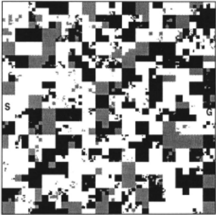
The four algorithms were compared on planning problems of varying size. Each environment was square, consisting of a start state in the center of the left wall and a goal state in center of the right wall. Each environment consisted of a mix of map obstacles known to the robot before the traverse and unknown obstacles measurable by the robot's sensor. The sensor used was omnidirectional with a 10-state radial field of view. Figure 6 shows an environment model with approximately 100,000 states. The known obstacles are shown in grey and the unknown obstacles in black.
The results for environments of 10 4 , 10 5 , and 10 6 states are shown in Table 1. The reported times are CPU time for a Sun Microsystems SPARC-10 processor. For each environment size, the four algorithms were compared on five randomly-generated environments, and the results were averaged. The off-line time is the CPU time required to compute the initial path from the goal to the robot, or in the case of FD*F, from the goal to all states in the environment. This operation is "off-line" since it could be performed in advance of robot motion if the initial map were available. The 0~-line time is the total CPU time for all replanning operatiOns needed to move the robot from the start to the goal.
| Focussed D* with Full Init | Focussed D* with Min Init | Basic D* | Brute-Force Replanner | |
|---|---|---|---|---|
| Off-line: 10 4 | 1.85 sec | 0.16 sec | 1.02 sec | 0.09 sec |
| On-line: 10 4 | 1.09 sec | 1.70 sec | 1.31 sec | 13.07 sec |
| Off-line: 10 5 | 19.75 sec | 0.68 sec | 12.55 sec | 0.41 sec |
| On-line: 10 5 | 9.53 sec | 18.20 sec | 16.94 sec | 11.86 min |
| Off-line: 10 6 | 224.62 sec | 9.53 sec | 129.08 sec | 4.82 sec |
| On-line: 10 6 | 10.01 sec | 41.72 sec | 21.47 sec | 50.63 min |
The results for each algorithm are highly dependent on the complexity of the environment, including the number, size, and placement of the obstacles, and the ratio of known to unknown obstacles. For the test cases examined, all variations of D* outperformed BFR in on-line time, reaching a speedup factor of approximately 300 for large environments. Generally, the performance gap increased as the size of the environment increased. If the user wants to minimize on-line time at the expense of off-line time, then FD*F is the best algorithm. In this algorithm, path costs to all states are computed initially and only the cost propagations are focussed. Note that FD*F resulted in lower on-line times and higher off-line times than BD*. The FD*M algorithm resulted in lower off-line times and higher on-line times than BD*. Focussing the search enables a rapid start due to fewer state expansions, but many of the unexplored states must be examined anyway during the replanning process resulting in a longer execution time. Thus, FD*M is the best algorithm if the user wants to minimize the total time, that is, if the off-line time is considered to be on-line time as well.
Thus, the Focussed D* algorithm can be configured to outperform Basic D* in either total time or the on-line portion of the operation, depending on the requirements of the task. As a general strategy, focussing the search is a good idea; the only issue is how the computational load should be distributed.
7 Conclusions
This paper presents the Focussed D* algorithm for real-time path replanning. The algorithm computes an initial path from the goal state to the start state and then efficiently modifies this path during the traverse as arc costs change. The algo rithm produces an optimal traverse, meaning that an optimal path to the goal is followed at every state in the traverse, assuming all known information at each step is correct. The focussed version of D* outperforms the basic version, and it offers the user the option of distributing the computational load amongst the on- and off-line portions of the operation, depending on .the task requirements. The addition of a heu ristic focussing function to D* completes its development as a generalization of A* to dynamic environments--A* is the special case of D* where arc costs do not change during the traverse of the solution path.
Acknowledgments
The author thanks Barry Brumitt and Jay Gowdy for feed back on the use of the algorithm.
@inproceedings{ijcai1995p213,
  title     = {The Focussed D* Algorithm for Real-Time Replanning},
  author    = {Stentz, Anthony},
  booktitle = {Proceedings of the Fourteenth International Joint Conference on
               Artificial Intelligence, {IJCAI-95}},
  publisher = {International Joint Conferences on Artificial Intelligence},
  editor    = {Chris S. Mellish},
  pages     = {1662--1668},
  year      = {1995},
  note      = {Planning},
  url       = {https://ijcai.org/proceedings/1995/213},
}
TY - CPAPER TI - The Focussed D* Algorithm for Real-Time Replanning AU - Stentz, Anthony T2 - Proceedings of the Fourteenth International Joint Conference on Artificial Intelligence, IJCAI-95 PB - International Joint Conferences on Artificial Intelligence PY - 1995 SP - 1662 EP - 1668 UR - https://ijcai.org/proceedings/1995/213 ER -Copied
Machine-readable versions of this paper, for tools and AI agents:





