Scalable Diagnosability Checking of Event-Driven Systems

1 Introduction

Nowadays, monitoring and diagnosing complex communicating event-driven systems has huge economic impact by ensuring better reliability, maintenance and safety [Lamperti and Zanella, 2003]. Such diagnostic capabilities are, for instance, required in aeronautic [Ghelam et al., 2006] or automotive systems, telecommunications [Pencol´e and Cordier, 2005] and electronic commerce [Yan et al., 2005]. For many years, the problem of automated fault diagnosis of these kinds of systems has received constant and considerable attention from researchers in the fields of Artificial Intelligence and Control. Given a monitor continuously receiving observations from a system, automated diagnosis methods aim at detecting all possible faults that explain the observations.

However, the resulting diagnosis depends on the diagnosability of the system [Sampath et al., 1995]. If the system is strongly diagnosable, a diagnostic process will find an accurate explanation for any possible set of observations from the system, otherwise the diagnosis will provide an ambiguous and useless explanation. Consequently, diagnosability analyses should be performed on the system before any diagnostic reasoning. The diagnosability results then help in choosing the type of diagnostic algorithm that can be performed and provide some information of how to change the system to make it more diagnosable [Pencol´e, 2004].

∗This research was supported by National ICT Australia (NICTA) in the framework of the SuperCom project (Model-Based Supervision of Composite Systems). NICTA is funded through the Australian Government's Backing Australia's Ability initiative, in part through the Australian National Research Council.

In this paper, we propose a formal framework for checking diagnosability on event-driven systems which is mainly motivated by two facts. On the one hand, checking diagnosability means determining the existence of two behaviours in the system that are not distinguishable. However, in realistic systems, there is a combinatorial explosion of the search space that forbids the practical use of classical and centralised diagnosability checking methods [Sampath et al., 1995] like the twin plant method [Jiang et al., 2001; Yoo and Lafortune, 2002]. On the other hand, in the case of a nondiagnosable system, checking its diagnosability is not sufficient; the diagnosability analysis should also provide the reasons why the system is not diagnosable. Given these reasons, either the system specification is redesigned or diagnostic reasoning is improved by taking into account the fact that the diagnosis of a fault may always be ambiguous.

Our proposal makes three contributions to the diagnosability problem. The first one is the definition of a new theoretical framework where the diagnosability problem is described as a distributed search problem. Instead of searching for not distinguishable behaviours in a global twin plant, we propose to distribute the search based on local twin plants and to determine such global behaviours without computing any part of the global twin plant. The second contribution comprises the nature of the feedback in case the faults are not diagnosable. Since the search is distributed over the whole system, the analysis provides an exhaustive and synthetic view of the diagnosability analysis of the system (why a given fault is not diagnosable). The third contribution is about the practical use of the algorithm. Since the diagnosability analysis problem is complex, the complete analysis may not be possible due to a lack of computational resources. However, the distributed search makes the computation scalable in the sense that our algorithm is able to provide an approximate but exhaustive solution to the diagnosability problemwhatever the computational resources are.

The paper is organised as follows. Section 2 presents some background on diagnosability on event-driven systems. Section 3 introduces our theoretical framework for diagnosability checking. Section 4 presents a scalable algorithm for distributed diagnosability checking. In section 5, related works are compared and discussed.

2 Background

2.1 Diagnosability in discrete-event systems

The system is modelled using classical automata: this formalism is aimed at modelling any discrete event system with multiple faults [Sampath et al., 1995]. We call a fault or a critical event any event whose occurrence a monitoring agent aims to identify. We suppose that a fault is not observable and occurs in one component. The modelling of the system is modular: each component has a local model and a synchronisation operator Sync is defined in order to implicitly represent the global model of the system.

Definition 1 (Model of a component) The model of the component i is the finite state machine Gi = 〈Xi, Σi, x0i , Ti〉, where

• Xi is the set of states (Xi = {x1i , . . . , xmi }),
• Σi is the set of events,
• x0i is the initial state, and
• Ti is the transition set (Ti ⊆Xi ×Σi ×Xi).

The set of events Σi is divided into four disjoint parts: Σoi is the set of observable events, Σsi is the set of events shared among components (they represent communications between components), Σfi is the set of unobservable fault events and Σui is the set of other unobservable events.

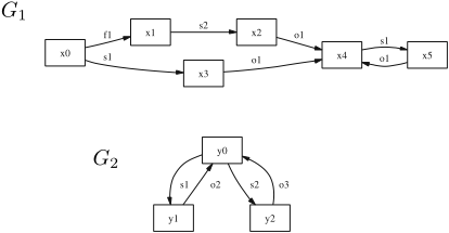
Figure 1 illustrates a system composed of two local models defined as above. The synchronisation operation, denoted Sync({M1, . . . ,Mn}, S), is the classical synchronisation operation on the n finite state machines {Mi} based on the set of shared events S. The result M of the synchronisation is the subset of the Cartesian product M1 × . . . ×Mn restricted with the following rules.

• If e ∈ S then from any state (x1, . . . , xn), the event e can occur if for all machines Mj where e can occur, there exists in Mj a transition xj e-→ x′j .
• If e ̸∈ S then from any state (x1, . . . , xn), the event e can occur if there exists a machine Mj where there exists a transition xj e-→ x′j .

The models of components and the operation Sync define the decentralized model of the system. The global model G then results from the synchronised product of the n components {Gi} where the shared events are synchronised:

A behaviour of the system is then represented by a transition path in G starting from the initial state x0 = (x01 , . . . , x0n ) of G. In the following, a path will always denote a transition path starting from the initial state. Moreover, as in [Sampath et al., 1995], the observable behaviour of the system is supposed to be live, which means that for any infinite path p of G, the sequence of observable events associated with p and denoted obs(p), is infinite.

The classical diagnosability property of the system is a global property defined on the paths in G [Sampath et al., 1995]. Two paths p and p′ in G are distinguishable iff obs(p) ̸= obs(p′ ). Let p = pFsF denote a path such that pF is a path ending with the occurrence of a fault F to a state xF and sF is a subpath whose initial state is xF . The diagnosability of fault F is then defined as follows:

Definition 2 F is diagnosable iff

If a fault is diagnosable then a diagnostic algorithm can diagnose its occurrence with certainty based on a finite sequence of observations. Diagnosability checking thus requires the search for an infinite path p′ , i.e. a path containing a cycle, with obs(p) = obs(p′ ) such that F is not in p′ . The pair (p, p′ ) is called a critical pair [Cimatti et al., 2003].

2.2 Twin plant method for checking diagnosability

We now recall a centralised method to check whether F is diagnosable or not: the twin plant method [Jiang et al., 2001]. For the sake of clarity in the rest of the paper, the twin plant method is presented in an original manner, based on the decentralised model instead of the global model.

Definition 3 (Local diagnoser) The local diagnoser of a component Gi is the nondeterministic finite state machine ˜Gi = 〈 ˜Xi, ˜Σi, ˜ x0i , ˜ Ti〉 where

• ˜Xi is the set of states ( ˜Xi ⊆ Xi × F with F ⊆ 2Σfi ),
• ˜Σi is the set of events ( ˜Σi = Σoi ∪ Σsi ),
• ˜ x0i = (x0i , ∅) is the initial state, and
• ˜ Ti ⊆ ˜Xi × ˜Σi × ˜Xi is the transition set (x,F) σ-→ (x′ ,F ′ ) such that there exists a transition sequence x σ1 -→ x1 · · · σm --→ xm σ-→ x′ in Gi with Σ′i = {σ1, . . . , σm} ⊆ Σfi ∪Σui and F ′ = F ∪ (Σ′i ∩ Σfi ).

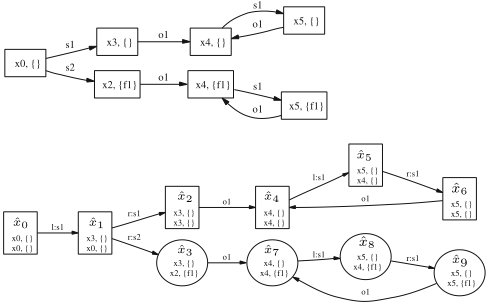
The top of Figure 2 depicts such a local diagnoser. The basic idea of a twin plant is to build a machine that compares every pair of paths (p, p′ ) in the system that have the same observable behaviour, i.e. obs(p) = obs(p′ ). A local twin plant is essentially the same type of machine but the paths are local to a component. A local twin plant is based on the synchronisation of two instances ˜Gli (left) and ˜Gri (right) of the same diagnoser based on the observable events Σoi = Σloi = Σroi . Since only observable behaviours are compared, the shared events must be distinguishable in both instances: in ˜Gli (resp. ˜Gri ), any shared event σ ∈ Σsi from ˜Gi is renamed l:σ ∈ Σlsi (resp. r:σ ∈ Σrsi ).

Definition 4 (Local twin plant) The local twin plant of Gi is the finite state machine

One state of a local twin plant is a couple ˆx = ((xl ,F l ), (xr ,F r )) that represents two possible diagnoses (the left one and the right one) given the same observable sequence. If F belongs to F l ∪F r but is not in F l ∩F r then F cannot be diagnosed in this state with certainty. In this case, the state ˆx is called F-nondiagnosable. Otherwise it is called F-diagnosable. Figure 2 illustrates a local twin plant for the diagnoser shown at the top of the same figure. Its state labels (top) are composed of the state labels of ˜Gl1 (middle) and ˜Gr1 (bottom). Circular nodes denote f1-nondiagnosable states.

In the following, ω represents any set of components Gω = {Gj1 , . . . , Gj|ω| } of the system with |ω| ≥ 1. The ω-coupled twin plant is the twin plant of ω obtained by synchronisation of the local twin plants.

Definition 5 (ω-coupled twin plant) The ω-coupled twin plant is

By extension, a state ˆx = (ˆxj1 , . . . , ˆ xj|ω| ) is called Fnondiagnosable if there exists a state ˆxjm which is locally F-nondiagnosable.

The synchronisation operation Sync is commutative and associative, moreover Σlsi , Σrsi and Σoi are disjoint sets by definition. Therefore any ω-coupled twin plant can be also obtained by first synchronising the local diagnosers over the set of shared events, to obtain the diagnoser of ω, followed by the synchronisation of two instances of the later over the set of observable events.

Consequently, considering ω = G = {G1, . . . ,Gn} the G-coupled twin plant represents exactly the global twin plant (GTP for short) of the system where all paths of G with the same observable behaviour are compared, hence the following fundamental result.

Theorem 1 F is diagnosable in G iff, in the G-coupled twin plant, there is no path p with a cycle containing at least one observable event and one F -nondiagnosable state.

Such a path p represents a critical pair (p1, p2): in the following, p is called a critical path. The twin plant method searches for such a path in the GTP.

3 Theoretical framework

We now show how to distribute the diagnosability check for a fault F without computing the GTP. The component where F may occur is denoted GF in the following. The terms diagnosable and nondiagnosable respectively denote F-diagnosable and F-nondiagnosable. Furthermore, Sync(G) denotes, without ambiguity, the product of all finite state machines in G synchronised over their shared events only.

Considering the set of local twin plants { ˆG1, . . . , ˆGn} defined in section 2, only ˆGF contains diagnosability information about F. The main idea of the distributed checking is to propagate firstly the diagnosability information to the other local twin plants. After the propagation, it is possible to decide locally which parts of the local twin plants are relevant to solve the diagnosability problem. Finally, for each local twin plant, a reduced twin plant is computed by removing all irrelevant parts.

3.1 Propagation of diagnosability information

The propagation of the diagnosability information from ˆGF to all other local twin plants is based on their connectivity with respect to ˆGF .

Definition 6 (α-connectivity Con(α, γ)) The set of finite state machines connected to the finite state machine γ by distance α is recursively defined as follows. Con(0, γ) = {γ}

Components γ1 and γ2 are connected if γ1 ∈ Con(1, γ2). The set transCon(γ) denotes the set of components whose behaviour can possibly influence that of γ (transCon(γ) =

⋃n-1 α=0 Con(α, γ)) where n is the number of components in the system.

Reducing a local twin plant ˆGi consists in finding a set of states, denoted P( ˆGi), that can possibly be involved in the nondiagnosable states of GTP. These possibly nondiagnosable states P( ˆGi) are determined by analysing the connectivity between the component Gi and the component GF .

Definition 7 (Possibly nondiagnosable states) The set of possibly nondiagnosable states P( ˆGi) of a local twin plant ˆGi is determined as follows.

1. P( ˆGi) = {x ∈ ˆXi | x is nondiagnosable} if Gi ∈ Con(0, GF ) (i.e. Gi = GF )
2. P( ˆGi) = ˆ Yi if Gi ∈ Con(α, Gf ) with α ∈ N+ and for all states ˆ y ∈ ˆ Yi and all connected twin plants Gj ∈ Con(α - 1, GF ) there exists a state (ˆ yi, ˆxj) in the twin plant Sync({ ˆGi, ˆGj}) such that ˆ xj is possibly nondiagnosable.

This definition can then be extended to any state ˆx = (ˆxj1 , . . . , ˆ xj|ω| ) from any ω-coupled twin plant:

Definition 8 A state ˆ x = (ˆxj1 , . . . , ˆxj|ω| ) in a ω-coupled twin plant ˆGω is possibly nondiagnosable iff

For example, to propagate the diagnosability information of f1 in G1 to G2 (see Figure 1) we compute ˆG1, the local nondiagnosable states (see Figure 2) and finally the twin plant ˆG2 (see Figure 3). Since ˆG1 and ˆG2 share the events l:s1 and r:s1 they are connected ( ˆG2 ∈ Con(1, ˆG1)). Thus to obtain P( ˆG2), a synchronisation of ˆG1 and ˆG2 leading to ˆG′ is required (see Figure 3). In ˆG′ only states (ˆx3, ˆ y3) and (ˆx7, ˆ y3) are composed of a state in P( ˆG1). Thus only state ˆ y3 could be possibly nondiagnosable. Since ˆG1 is the only connected twin plant in Con(1 - 1, ˆG1) there is no need to consider other local twin plants to check whether ˆ y3 is indeed in P( ˆG2). Therefore the set of possibly nondiagnosable states in ˆG2 is P( ˆG2) = {ˆ y3}.

Every state that is not possibly nondiagnosable is certainly diagnosable. This results from the following relationship between nondiagnosable and possibly nondiagnosable states of the GTP:

Theorem 2 A state ˆx in the GTP is nondiagnosable iff it is possibly nondiagnosable.

Proof:

• (⇒) Suppose there exists a state ˆx = (ˆx1, . . . , ˆxn) in the GTP such that ˆ x is nondiagnosable and a state ˆxi such that ˆ xi /∈ P( ˆGi). Cond. 3 of def. 7 implies that ˆGi is in transCon( ˆGF ). Since ˆx is nondiagnosable the state ˆ xF from lows that ˆ xF ∈ P( ˆGF) (see cond. 1 of def. 7), so ˆGi is in transCon( ˆGF ) \ { ˆGF}. Therefore, there exists an α > 1 such that

ˆGF , also contained in ˆx, is nondiagnosable. It folˆGi ∈ Con(α, ˆGF ). Cond. 2 of def. 7 ensures that there is a twin plant ˆGj ∈ Con(α-1, ˆGF ) in which all states ˆx′j , for which (ˆx′j , ˆxi) is in Sync({ ˆGj , ˆGi}), do not belong to P( ˆGj ). Since GTP results from the synchronisation of ˆGj and ˆGi, it means that ˆ xi /∈ P( ˆGi) implies that ˆ xj /∈ P( ˆGj ) where ˆxj denotes the state from ˆGj contained in ˆ x. The previous reasoning led from the existence of a state ˆxi = ˆ yα in a twin plant ˆGi = ˆHα ∈ Con(α, ˆGF ) with ˆ yα /∈ P( ˆHα) to the existence of a state ˆxj = ˆ yα-1 in a twin plant ˆGj = ˆHα-1 ∈ Con(α - 1, ˆGF ) with ˆ yα-1 /∈ P( ˆGα-1). By recursively applying α - 1 times the same reasoning, it follows that there exists a twin plant ˆH0 belonging to Con(0, ˆGF ) and a state ˆ y0 from ˆH0 belonging to ˆx such that ˆ y0 /∈ P( ˆH0). Since ˆGF is the only element in Con(0, ˆGF ) (see def. 6) it means that ˆH0 is actually ˆGF and ˆ y0 = ˆ xF . It finally follows that ˆ xF /∈ P( ˆGF ), which is a contradiction.

• (⇐) Suppose there exists a state ˆx ∈ P(GTP) containing the local state ˆ xF ∈ ˆGF such that ˆx is diagnosable. This implies that ˆ xF /∈ P( ˆGF). Therefore ˆ x /∈ P(GTP) (see def. 7) which contradicts the assumption. □

3.2 Distributed diagnosability verification

We now show how we can exploit Theorem 2 firstly to reduce the size of twin plants by removing all states that are irrelevant to the diagnosability test (see Lemma 1 below) and secondly to distribute the diagnosability test to a set of twin plants.

Definition 9 (Reduced twin plant) A twin plant is reduced if all its states are either initial or on a path whose target state is possibly nondiagnosable.

In the following, R( ˆG) denotes the twin plant that is obtained by removing all states ˆx /∈ P( ˆG) of ˆG that do not lead to a possibly nondiagnosable state. To simplify the synchronisation of reduced twin plants the event set of the latter remains unchanged (R( ˆΣ) = ˆΣ), that is, even if R( ˆG) does not contain any transitions labelled ˆσ ∈ ˆΣ, the event still belongs to its event set. Thus the following equivalence holds for any two twin plants ˆG, ˆG′ : R(Sync({ ˆG, ˆG′ })) = R(Sync({R( ˆG), R( ˆG′ )})) (see also def. 7).

Lemma 1 The global twin plant ˆG = Sync({ ˆG1, . . . , ˆGn}) contains exactly the same critical paths as R( ˆG).

Proof: Since the target state of every critical path p in ˆG is part of a cycle containing at least one nondiagnosable state ˆx (see Theorem 1), every state in p leads to ˆx and hence to a state that is entirely composed of possibly nondiagnosable states. Thus, p is also a path in R( ˆG). Further, since every path in R( ˆG) is also a path in ˆG it follows that R( ˆG) contains only the critical paths defined in ˆG. □

We now show how we can decide the diagnosability problem based on a set of distributed twin plants without requiring the computation of the GTP.

Theorem 3 A fault F in system G is diagnosable iff there exists a set of reduced twin plants ˆGR = { ˆGω1 , . . . , ˆGωk } such that

1. {ω1, . . . , ωk} is a partition of the system components (⋃ki=1 ωi = G and ωi ∩ ωj = ∅ for all ωi ̸= ωj) and
2. no plant in ˆGR contains an observable possibly nondiagnosable cycle (OPNC for short) (i.e. a path p = ˆx ˆσ-→ ˆx′ · · · ˆσ′′ --→ ˆx with at least one possibly nondiagnosable state and one observable transition label).

Proof:

• (⇒) Suppose F is diagnosable, but there does not exist such a set GR. The GTP, which satisfies cond. 1, also contains an OPNC and thus an observable nondiagnosable cycle (see Theorem 2). This implies that F is not diagnosable (see Theorem 1) and thus contradicts the assumption.
• (⇐) Suppose now that there exists such a set GR and F is not diagnosable. From the nondiagnosability of F it follows that there exists an observable nondiagnosable cycle in the GTP and hence an OPNC with an observable event σ ∈ Σoi (see Theorem 2). Based on the synchronisation operation (see page 2) it means that every ω-coupled twin plant ˆGω with Gi ∈ ω contains an OPNC. Thus every set satisfying cond. 1, and therefore involving Gi, does not satisfy cond. 2. Hence there does not exists such a set GR which contradicts the assumption. □

4 Algorithm

This section presents a scalable algorithm that exploits Theorem 3 to reduce the search space of the diagnosability analysis by distributing it on several reduced twin plants. Every set of reduced twin plants GR represents a partition of the components of the system and the challenge is to find one that contains no OPNCs and thus proves that F is diagnosable. OPNCs can be removed by synchronising connected twin plants. Therefore this operation is the basis for the distributed diagnosability check (see Algorithm 1).

The algorithm performs as follows. After the initialisation and the computation of the local reduced twin plants (line 3-5), the basic idea is to synchronise them pairwise using the function Sync(R( ˆGi ), R( ˆGi′ )). The synchronisation is performed only if either R( ˆGi ) or R( ˆGi′ ) has an OPNC. This pairwise synchronisation and the reduction of the resulting twin plant is computed using function RedP airwiseSync( ˆG) (line 7). The selection of pairs to synchronise is important since it has a strong impact on the algorithm efficiency. Among the different selection heuristics, e.g. [Lamperti and Zanella, 2003], [Pencol´e and Cordier, 2005], a common rule must be respected: a pair of twin plants to synchronise must be connected otherwise the synchronisation will not remove OPNCs.

The synchronisation operation is repeated step by step until the algorithm stops due to one of the following causes.

1. None of the twin plants in ˆG contains an OPNC, that is, a partition GR has then been determined which verifies that fault F is diagnosable (see Theorem 3).
2. A twin plant contains an OPNC that cannot be removed by further synchronisations. This is the case if the reduced GTP has been computed which involves all components.
3. Due to finite computational resources, the algorithm must stop. In this case it returns a set of twin plants with OPNCs that provides all possible reasons of why F might not be diagnosable. At this level, the nondiagnosability of F is not certain but it can be deduced that any subset of components involved in an element of the partition is not sufficient to diagnose F with certainty.

Algorithm 1 Distributed diagnosability check

• 1: INPUT:
• component models G1, . . . Gn of the system
• fault F that can occur in component GF
• 2: Initialisations: ˆG ← ∅

Set of relevant twin plants

• 3: Compute local twin plants ˆGi for all components Gi and add them to ˆG
• 4: ˆG ← GetNonDiagStateLab( ˆG, ˆGF )
• 5: Reduce all twin plants in ˆG
• 6: while ExistsOPNC( ˆG), and SufficientMemory( ˆG) and NrElements( ˆG) > 1 do
• 7: ˆG ← RedP airwiseSync( ˆG)
• 8: end while
• 9: if ExistsOPNC( ˆG) is false then
• 10: return "F is diagnosable"
• 11: else
• 12: ˆGcyc ← GetT P sW ithOP NC( ˆG)
• 13: return ˆGcyc
• 14: end if

In case (2), that is if F is not diagnosable, all critical paths are returned. They provide a complete diagnosability analysis of the undistinguishable behaviours that cause the nondiagnosability of F . This information also contains a synthetic view of the nondiagnosability of F .

Extracting this synthetic view from the OPNCs

((xlj|ω| , F l j|ω| ), (xrj|ω| , F r j|ω| )) in the OPNCs. If one label contains F (i.e. F l = ⋃|ω| i=1 F l i ) and the other label is empty (i.e. F r = ⋃|ω| i=1 F r i = ∅) it means that there exists an infinite nominal behaviour in the system which cannot be distinguished from a faulty behaviour. In this case, the observation of the system does not guarantee that a fault can be detected, it must be updated (respecified) in order to guarantee the diagnosability of F. If the label F r is not empty, then the diagnosability problem results from the fact that the occurrence of the faults F r cannot be discriminated from the occurrence of F. In this case, a designer can decide that the discrimination of F with F r is not important and abstract the set of faults to only diagnose a fault Fabs = F ∨ F r .

5 Discussion

Diagnosability on DES is a problem that has been introduced in [Sampath et al., 1995] where the authors solve it by detecting some transition cycles of ambiguous states in a global diagnoser. The global diagnoser is equivalent to the determination of the local diagnoser (see Definition 3) where the global model G is seen as a component. The main drawback of this method results from the diagnoser computation which is exponential in the number of states in the global model (determination) and as a consequence is doubly exponential in the number of components in the system. [Jiang et al., 2001; Yoo and Lafortune, 2002] then propose new algorithms which are only polynomial in the number of states in G and which introduce the twin plant method. The question of efficiency is raised in [Cimatti et al., 2003] where the authors propose to use symbolic model-checking to test a restrictive diagnosability property by taking advantages of efficient model-checking tools. But, still the diagnosability problem is seen as a test on a system and not as a deep analysis of the reasons why a system is not diagnosable. In [Pencol´e, 2004], the author introduces the problem of analysing diagnosability of a system in a decentralised way by aggregating local non reduced twin plants until a critical path is detected. In this method, the diagnosability analysis is not scalable and only partial since the feedback is just about the detected critical path.

6 Conclusion and future work

Our theoretical framework solves the diagnosability problem in a distributed manner and takes into account the distributed nature of complex event-driven systems. We have also proposed an algorithm that is scalable in the sense that, if the problem is too complex to be solved with available computational resources, it can still provide an approximate analysis of the diagnosability of the system. In case of a negative answer to the diagnosability problem, we claim that finding a counter example is not sufficient to assist any designer of a system to improve diagnosability. We thus propose a synthetic view of the diagnosability results that summarise the different reasons why a fault is not diagnosable.

The perspectives of this work are numerous: it is a clear first step to assist any designer to make diagnosable systems because of the synthetic view of the results instead of a single counter example. One of our next challenge is the application of this framework to provide design recommendations for improving the diagnosability of health monitoring system for aircraft maintenance [Ghelam et al., 2006] or to provide an assistance to the design of composite Web Services [Yan et al., 2005]. Another challenge is to improve our algorithm in order to search for optimal partitions where each element of the partition is as small as possible. From an optimal partition, we can then derive optimal diagnostic algorithms based on set of small system parts that still guarantee an accurate global diagnosis.

Acknowledgments

The authors thank Jussi Rintanen, Alban Grastien and the anonymous reviewers for useful discussions and comments.