
Hierarchical Diagnosis of Multiple Faults
Proceedings of the Twentieth International Joint Conference on Artificial Intelligence. Pages 581-585.
© 2007 International Joint Conferences on Artificial Intelligence
Abstract
Due to large search spaces, diagnosis of combinational circuits is often practical for finding only single and double faults. In principle, system models can be compiled into a tractable representation (such as DNNF) on which faults of arbitrary cardinality can be found efficiently. For large circuits, however, compilation can become a bottleneck due to the large number of variables necessary to model the health of individual gates. We propose a novel method that greatly reduces this number, allowing the compilation, as well as the diagnosis, to scale to larger circuits. The basic idea is to identify regions of a circuit, called cones, that are dominated by single gates, and model the health of each cone with a single health variable. When a cone is found to be possibly faulty, we diagnose it by again identifying the cones inside it, and so on, until we reach a base case. We show that results combined from these hierarchical sessions are sound and complete with respect to minimum-cardinality diagnoses. We implement this method on top of the diagnoser developed by Huang and Darwiche in 2005, and present evidence that it significantly improves the efficiency and scalability of diagnosis on the ISCAS-85 circuits.
- [Bryant, 1986] Randal E. Bryant. Graph-based algorithms for Boolean function manipulation. IEEE Transactions on Comput- ers, 35(8):677-691, 1986.
- [Darwiche, 2001] Adnan Darwiche. Decomposable negation nor- mal form. Journal of the ACM, 48(4):608-647, 2001.
- [Feldman and van Gemund, 2006] A. Feldman and A.J.C van Gemund. A two-step hierarchical algorithm for model-based di- agnosis. In AAAI, 2006.
- [Hansen et al., 1999] Mark C. Hansen, Hakan Yalcin, and John P. Hayes. Unveiling the ISCAS-85 benchmarks: A case study in reverse engineering. IEEE Design and Test of Computers, 16(3):72-80, 1999.
- [Huang and Darwiche, 2005] Jinbo Huang and Adnan Darwiche. On compiling system models for faster and more scalable diag- nosis. In AAAI, pages 300-306, 2005.
- [Kirkland and Mercer, 1987] T. Kirkland and M. R. Mercer. A topological search algorithm for ATPG. In DAC, pages 502-508, 1987.
- [Lu et al., 2003a] Feng Lu, Li-C. Wang, K.-T. (Tim) Cheng, John Moondanos, and Ziyad Hanna. A signal correlation guided ATPG solver and its applications for solving difficult industrial cases. In DAC, pages 436-441, 2003.
- [Lu et al., 2003b] Feng Lu, Li-C. Wang, Kwang-Ting Cheng, and Ric C-Y Huang. A circuit SAT solver with signal correlation guided learning. In DATE, pages 10892-10897, 2003.
- [Smith et al., 2004] Alexander Smith, Andreas Veneris, and Anas- tasios Viglas. Design diagnosis using Boolean satisfiability. In ASP-DAC, pages 218-223, 2004.
- [Torta and Torasso, 2004] Gianluca Torta and Pietro Torasso. The role of OBDDs in controlling the complexity of model-based di- agnosis. In DX, 2004.
References were extracted automatically from the PDF and may contain errors.
Full text extracted automatically from the PDF; figures, tables and equations may differ. The PDF is the version of record.
1 Introduction
In this work we consider fault diagnosis of combinational circuits, where the observed (abnormal) input and output values of a circuit, together with its implementation, are given to a diagnosis engine, which finds possible sets of faulty gates that explain the observation.
A diagnosis tool implementing a model-based approach was recently presented in [Huang and Darwiche, 2005], where systems to be diagnosed are modeled as propositional formulas in conjunctive normal form (CNF), which are then compiled into decomposable negation normal form (DNNF) [Darwiche, 2001]. This tool, which we shall refer to as HD05, was shown particularly to improve in efficiency and scalability over an earlier tool [Torta and Torasso, 2004] based on compiling system models into ordered binary decision diagrams (OBDD) [Bryant, 1986].
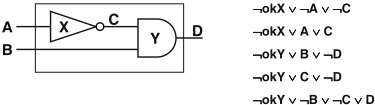
Consider the example in Figure 1, reproduced from [Huang and Darwiche, 2005]. HD05 models the circuit as a propositional formula where each signal of the circuit translates into a propositional variable (A, B, C, D). For each gate an extra variable (okX, okY ) is introduced to model its health. The propositional formula is such that when all health variables are true, the remaining variables are constrained to model the functionality of the gates. For instance, the first two clauses shown in the figure are equivalent to the sentence okX ⇒ (A ⇔ ¬C), modeling the health of the inverter X.
Given a (typically abnormal) valuation of the inputs and outputs of the circuit, called an observation, a (consistencybased) diagnosis is then a valuation of the health variables that is consistent with the observation and system model. For instance, given the observation ¬A ∧ B ∧ ¬D, one diagnosis is ¬okX ∧ okY , meaning that the inverter X is broken and the and-gate is healthy. It is known that once the system model is compiled into DNNF, one can compute a compact representation of all diagnoses in time linear in the size of the DNNF [Darwiche, 2001].
A major advantage of HD05 is that DNNF is known to be a strictly more succinct representation than OBDD and supports efficient algorithms that compute diagnoses of arbitrary cardinality as well as minimum cardinality [Darwiche, 2001]. When this approach is applied to large circuits, however, compilation of system models into DNNF can become a bottleneck due to large numbers of health variables.
We propose a solution to this problem based on hierarchical diagnosis. We start with an abstraction of the circuit where certain regions of the circuit, called cones, are "carved out" based on a structural analysis. The abstract model, being generally much simpler, allows larger circuits to be compiled and their diagnoses computed. The cones are diagnosed only when they are identified by the top-level diagnosis as possibly faulty. We discuss the intricacies involved in properly diagnosing the cones so that redundancy is avoided and results combined from the hierarchical diagnosis sessions are sound and complete with respect to minimum-cardinality diagnoses.
We implement our new approach on top of HD05. Using ISCAS-85 benchmark circuits, we show that we can now diagnose some circuits (with arbitrary fault cardinality) for the first time. For circuits that can already be handled by HD05, we also observe a significant improvement in diagnosis time.
2 Notation and Definitions
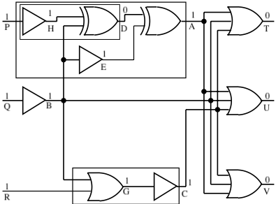
We shall use the circuit in Figure 2 as a running example. The numbers shown alongside the gate outputs are values of the signals, which can be ignored for the moment.
2.1 Circuits, Dominators, and Cones
We use C to denote the circuit as well as the set of gates of the circuit including the inputs (as trivial gates). We identify a gate with its output signal. The set of inputs of the circuit is denoted IC and the set of outputs OC. For example, IC = {P, Q, R} and OC = {T, U, V } for the circuit in Figure 2.
One may observe that certain regions of this circuit have only limited connectivity with the rest of the circuit. For example, the dotted box containing gates {A,D,E,H, P} is a sub-circuit that contributes a single signal (A) to the rest of the circuit. The box containing gates {D,H, P} is another such example. We refer to such a sub-circuit as a cone (also known as fan-out free formula [Lu et al., 2003b; 2003a]), which we now formally define.
The fan-in region of a gate G ∈ C is the set of all those gates that have a path passing through G going to some output gate. The fan-in region of gate A in Figure 2, for example, is {A, B, D, E, H, P, Q}.
Definition 1. (Dominator) A gate X in the fan-in region of gate G is dominated by G, and conversely G is a dominator of X, if any path from gate X to an output of the circuit contains G [Kirkland and Mercer, 1987].
The notion of cone then corresponds precisely to the set of gates dominated by some gate G, which we denote by ΔG. For example, the dotted box mentioned above corresponds to ΔA = {A, D, E, H, P }. From here on, when the meaning is clear, we will simply use G to refer to the cone rooted at G.
2.2 Abstraction of Circuit
A circuit can be abstracted by treating all maximal cones in it as black boxes (a maximal cone is one that is either contained in no other cone or contained in exactly one other cone which is the whole circuit). For example, cone A can be treated as a virtual gate with two inputs {P,B} and the output A. Similarly, cone A itself can be abstracted by treating cone D as a virtual gate. An abstraction of a circuit can hence be defined as the original circuit minus all non-root gates of maximal cones, or more formally:
Definition 2. (Abstraction of circuit) Given a circuit C, let C′ = C if C has a single output; otherwise let C′ be C augmented with a dummy gate collecting all outputs of Cs. The abstraction ΘC of circuit C is then the set of gates X ∈ C such that there is a path from X to the output O of C′ that does not contain any dominator of X other than X and O.
For example, ΘC = {T, U, V,A,B,C}. E ̸∈ ΘC as E cannot reach any output without passing through A, which is a dominator of E. Similarly, ΘA = {A, D, E}. H ̸∈ ΘA as its only path to A contains D, which is a dominator of H.
3 DNNF-based Diagnosis
Before presenting our new algorithm we briefly review the baseline diagnoser HD05 [Huang and Darwiche, 2005], which is based on compiling the system model (circuit in our case) from CNF to DNNF [Darwiche, 2001].
DNNF is a graph-based representation for propositional theories. Specifically, each DNNF theory is a DAG (directed acyclic graph) with a single root where all leaves are labeled with literals and all other nodes are labeled with either AND or OR; in addition the decomposability property must be satisfied: children of any AND-node must not share variables.
Once a system model is converted into DNNF, consistencybased diagnoses, as well as minimum-cardinality diagnoses, can be computed in time polynomial in the size of the DNNF [Darwiche, 2001]. The key is that decomposability allows nonobservables to be projected out in linear time, and allows diagnoses computed for children to be combined at a parent AND-node simply by cross-concatenation (note that diagnoses computed for children can naturally be unioned at a parent OR-node).
Our new algorithm aims to improve the efficiency and scalability of this approach in the context of circuit diagnosis. We will continue to model a circuit as a CNF formula and rely on DNNF compilation to compute diagnoses. The main innovation is a structure-based method to reduce the number of health variables required for the model and hence the difficulty of compilation, while maintaining the soundness and completeness of the diagnoser. In the rest of the paper we will assume that only minimum-cardinality diagnoses are sought.
4 Hierarchical Diagnosis
The key idea behind our new algorithm is to start by obtaining the abstraction ΘC of a circuit C as defined in Section 2, and then diagnose C pretending that only gates in ΘC could be faulty. This is the basic technique that will significantly reduce the number of health variables required in the system model, allowing us to compile and diagnose larger circuits. Once this top-level diagnosis session finishes, if a gate appearing in a diagnosis is the root of a cone, which has been abstracted out, then we attempt to diagnose the cone, in a similar hierarchical fashion.
Two things are worth noting here before we go into details. First, cones are single-output circuits and hence the diagnosis of cones will alway produce diagnoses of cardinality one. Second, the diagnosis of a cone is not performed simply with a recursive call as one may be tempted to expect. Indeed the later diagnosis sessions are very distinct from the initial toplevel session. The reason has to do with avoiding redundant computation, which we will discuss later in the section.
We now present in detail our hierarchical diagnosis algorithm, which we will refer to as HDIAG. Pseudocode of HDIAG is given in Algorithm 1.
4.1 Algorithm
Step 1 (dominators)
HDIAG starts by identifying the nontrivial dominator gates in the circuit (a trivial dominator is one that dominates only itself). First the dominators of every gate are obtained. The dominators of a gate are the gate itself union the intersection of the dominators of its parents [Kirkland and Mercer, 1987], which can be found by a simple breadth-first traversal of the circuit starting from the outputs. During this process the nontrivial dominators can be identified. FINDDOMINATORS implements this procedure on line 3 of Algorithm 1.
In our example, the dominator sets for T , U, V , A, B, C are {T}, {U}, {V}, {A}, {B}, {C}, respectively; the dominator set for D is {D,A} and for H is {H,D,A}. It can be easily seen that the gates T , U, and V are trivial dominators whereas D and A are nontrivial dominators.
Step 2 (cones and their inputs)
Each nontrivial dominator defines a cone that can be abstracted out. Next we identify the inputs of these cones by a depth-first traversal of the circuit. Suppose G is a cone. The inputs IG of G can be found by traversing the fan-in region of G so that if we reach either an input of the circuit or a gate that does not belong to ΔG, we add it to IG and backtrack. FINDCONES implements this procedure on line 3 of Algorithm 1.
For cone D in our example, we traverse the fan-in region of D in the order D,H, P,B. Gates P and B are added to the inputs of cone D. We backtrack from B as B ̸∈ ΔD. The inputs of cone D are thus {P, B}.
Step 3 (top-level diagnosis)
The rest of the algorithm proceeds in two phases. In the first phase we have the (abnormal) observation for the whole circuit. We first propagate the values of the inputs bottom-up, setting the (expected) value of each internal gate of the circuit. These values are saved for reference later. The observed outputs of the circuit are then set which may be abnormal. PROPAGATEINPUTS, SAVEVALUES, and SETOBSOUTPUTS on lines 4 and 5 of Algorithm 1 implement these procedures.
The health of the abstraction of the circuit, ΘC, is then diagnosed. This is achieved by associating a health variable with every gate in ΘC. ΘC contains all the domina-
Algorithm 1 HDIAG : Hierarchical Diagnosis Algorithm
function HDIAG ( C, Obs )
inputs: {C: circuit/set of gates}, {Obs: set of <gate,bool>}
output: {set of sets of gates}
local variables: {OC, IC,Π,T : set of gates},{Λ,D:set of sets of gates}, {Ω :<CNF, set of gates>}
- 1: OC ← OUTPUTS( C )
- 2: IC ← INPUTS( C )
- 3: FINDDOMINATORS(OC ), FINDCONES(OC )
- 4: PROPAGATEINPUTS ( C, IC,Obs ), SAVEVALUES ( C )
- 5: SETOBSOUTPUTS ( OC,Obs )
- 6: T← TRAVERSE ΘC ( OC, IC ), ATTACHOKS( T )
- 7: Ω←GENMODEL( C,OC ∪ IC )
- 8: Λ←CALLHD05( Ω,Obs ), ORDERBYDEPTH(Λ )
- 9: RESTOREVALUES ( )
- 10: D←φ
- 11: for all Π ∈ Λ do
- 12: D←D∪ FINDEQDIAGNOSES(Π )
- 13: return D
Algorithm 2 TRAVERSE ΘC : Traverses Top Level
function TRAVERSE ΘC ( OC, IC )
inputs: {OCIC, set of gates} output: {set of gates} local variables: {Q,K,T: set of gates}, {Y,O} : gate 1: O←SINGLEOUTPUT(OC ) 2: Q← {O}, T← φ 3: while ¬ISEMPTY (Q) do 4: Y ←POP( Q ) 5: if Y ̸∈ IC then 6: T←T∪ {Y } 7: if ¬ISDOMINATOR ( Y ) || Y ==O then 8: K←CHILDREN ( Y ), Q←Q∪K 9: return T
tors of the top-level hierarchy plus all the non-dominators that sit between those dominators and the outputs OC of the circuit. TRAVERSE ΘC traverses the top-level hierarchy of the circuit. SINGLEOUTPUT on line 1 of Algorithm 2 implements the attachment of dummy gate described in Definition 2. TRAVERSE ΘC is implemented so that as soon as it encounters an input of the circuit or a nontrivial dominator (other than root, see line 7 of Algorithm 2), it backtracks (the inputs are excluded as they are assumed to be healthy). ATTACHOKS associates health variables with each gate in this hierarchy.
Nowwe create an abstract systemmodel similar to the full model used in [Huang and Darwiche, 2005]. The abstract model contains a system description, in CNF, over the set of observables (IC ∪OC) and nonobservables (C\(IC ∪OC)). The model is generated by the function GENMODEL and returned as Ω. Note that only the clauses representing the gates marked by ATTACHOKS will have additional health variables. HD05 is then called with Ω and the observation to perform the diagnosis. The diagnoses thus obtained will be referred to as top-level diagnoses. If a nontrivial dominator G ∈ ΘC is reported to be possibly faulty, we then enter the second phase by diagnosing the cone under G.
For example, in Figure 2, given the inputs, all the outputs of the circuit should be 1, but, all of them are 0 in our ob-
Algorithm 3 FINDEQDIAGNOSES : Diagnosis of Cones
function FINDEQDIAGNOSES ( Π ) inputs: {Π, set of gates} output: {set of sets of gates} local variables: {E, Λ: set of sets of gates}, {P,R,C, IX,Q,T,S: set of gates}, {X, Y : gate}, {Ω :<CNF, set of gates>}, {Obs: set of <gate,bool>} 1: E← {Π}, D← {Π} 2: while ¬ISEMPTY( E ) do 3: P← POP( E ) 4: PROPAGATEFAULT ( P ) 5: for all X ∈ P such that X is a cone and is not the whole circuit do 6: if X ̸∈ Q then 7: Q←Q∪ {X} 8: C ← TRAVERSECONE ( X ), IX ← INPUTS ( C ) 9: T ← TRAVERSE ΘC ( {X}, IX ), ATTACHOKS ( T ) 10: Ω ← GENMODEL ( C, {X} ∪ IX ) 11: Obs ←VALUATION( {X} ∪ IX ) 12: Λ ← CALLHD05 ( Ω, Obs ), SETDIAGS( X, Λ ) 13: else 14: Λ ← DIAGS( X ) 15: for all R ∈ Λ do 16: Y ←POP ( R ) 17: if X ̸= Y then 18: S ← SUBSTITUTE ( X, Y, P ) 19: E←E ∪ {S}, D←D ∪ {S} 20: RESTOREVALUES ( ) 21: CLEARDIAGS(Q ) 22: return Dservation. We introduce health variables for the set of gates ΘC\IC = {T, U, V, A, B, C}, create a model of the abstraction of the circuit, and pass the model along with the observation ¬T ∧ ¬U ∧ ¬V ∧ P ∧ Q ∧ R to HD05. One of the diagnoses returned by HD05 is ¬okA∧¬okB ∧¬okC or, to use an alternative notation, {A, B, C} (in the rest of the paper we will use this latter notation expressing a diagnosis as a set of faulty gates). Since A is a cone, we enter the second phase.
Step 4 (diagnosis of cones)
Suppose that Π = {X,G1, . . . ,Gn} is a diagnosis found in the top-level phase and that X ∈ Π is (the root of) a cone. It should be clear that given the faulty output b of X, if there is a gate Y ∈ ΔX that, when assumed faulty, permits the same value b at X, then replacing X with Y will yield a valid global diagnosis. This way we try to expand our top-level diagnoses in the procedure FINDEQDIAGNOSES (line 12 of Algorithm 1), given in Algorithm 3.
Mainly, for each cone X in each top-level diagnosis Π, we find a diagnosis for X hierarchically. We identify X as a sub-circuit with the single output X and the inputs IX. The minimum cardinality of diagnoses for X is always one as we mentioned earlier. We then replace X with its singleton diagnoses, in Π, one by one, to produce new global diagnoses. This process is iterated until we reach a base case (no cones left to be diagnosed). We treat each Π and all diagnoses generated from it as a single class of diagnoses and use it to avoid redundant computation (explained in Section 4.2).
Cone X could be diagnosed as is done for the whole circuit but there is more to be done in order to find correct diagnoses.
Specifically, we need a set of values for the inputs and output of cone X as an observation to pass to HD05. First of all we restore expected values of the gates in the circuit (line 9 of Algorithm 1) before we call FINDEQDIAGNOSES.
We want to diagnose cone X under the assumption that all of the gates Gi ∈ Π are also faulty, so we need to propagate the fault effect of all Gi into the sub-circuit. Since faults in circuits propagate bottom-up, we put the set of gates in each diagnosis in decreasing order of their depth in the circuit (ORDERBYDEPTH on line 8 of Algorithm 1). A fault is processed simply by flipping the output of the faulty gate and propagating its effect. This is done for each G ∈ Π separately in the order in which they appear in Π. This has the desired effect of setting an observation across cone X (IX ∪ {X}) that is consistent with the observation of the overall circuit. Cone X is now ready for diagnosis.
Note that, again, only the abstraction ΘX of cone X is diagnosed. As we mentioned earlier, however, this is not simply a recursive call to Algoritm 1, but needs to be handled differently (Algorithm 3). TRAVERSECONE (line 8) identifies and returns the set of gates of the cone (i.e., ΔX). VALUATION returns a set of <gate, bool> pairs which represents the currently assigned values to the set of gates {X} ∪ IX passed as input (line 11). The returned set serves as an observation across the cone. Given the cone, its observables and nonobservables, the health of its abstraction is diagnosed using HD05 and the set of singleton diagnoses Λ found is saved (line 12). These diagnoses can be retrieved by DIAGS (line 14). SUBSTITUTE ( X, Y, P) generates a new diagnosis by replacing X with Y in P (line 18). Finally, we clear these diagnoses before returning from the function (line 21).
The diagnosis of cones is similar to that of the overall circuit given in Algorithm 1. There are, however, a few details worth mentioning: (i) Every cone is diagnosed hierarchically, i.e., for a cone X we diagnose only the top-level hierarchy ΘX of X. (ii) In a single call to FINDEQDIAGNOSES every cone is diagnosed once (ensured by line 6 of Algorithm 3). This is sufficient and will be explained later. (iii) Once a new diagnosis is generated by substitution, it is added to the set E for further processing (line 19 of Algorithm 3). (iv) The fault effect of a diagnosis is propagated before the diagnosis is processed, and undone afterwards. (v) As substitutions are made, the gates in a newly generated diagnosis may not have the depth order discussed above; however, we do not re-order them for reasons that will be clear soon.
Continuing with our example, we reorder {A,B,C} as {B,A,C}. We flip B to 0, propagate the effect that flips E to 0 and D to 1. A remains 1 at this stage; we then flip A to 0 (gate C is irrelevant to the diagnosis of cone A). Note that the correct output of cone A should be 1 given its inputs P(1) and B(0). We place health variables at the gates ΘA\IA = {A,D,E}, generate a model for cone A, and pass it to HD05 with the observation ¬A ∧ P ∧ ¬B, which returns three diagnoses of cardinality one: {A}, {D}, {E}. Note that {A} is a trivial diagnosis. Substituting D and E for A in the top-level diagnosis {B,A,C}, we get two new diagnoses: {B,D,C}, {B,E,C}.
4.2 Avoiding Redundancy
Since cones can be shared among different diagnoses, a cone is potentially visited more than once before all final diagnoses are computed. It may or may not be redundant to diagnose one cone multiple times. There are three cases to consider:
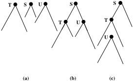
- Suppose that in a top-level diagnosis, a cone S appears in two diagnoses {S, T} and {S, U}, shown in Figure 3a. It can be seen that neither T nor U lies in the fan-in region of cone S. Thus no fault at T or U can affect values at the inputs or output of cone S. This means that diagnosis of S can be obtained once and can be used in the processing of both of the top-level diagnoses. This case is currently not implemented in our code.
- In Figure 3b, both T and U lie in the fan-in region of the cone S. Thus faults at T or U can affect values at the inputs and output of cone S. However, if we consider a fault at T and its effect across S (at the inputs and output of S), it may not be same as a fault at U and its effect across S. Thus the diagnosis of cone S during the processing of {S, T } may be completely different from that during the processing of {S, U}. Hence cone S has to be diagnosed twice in this case. This is why we clear the diagnoses before we return from FINDEQDIAGNOSES in Algorithm 3.
- In Figure 3c, we assume that only {S, T} is a top-level diagnosis whereas {S, U} is a diagnosis obtained during the processing of {S, T} such that {U} is a cardinality one diagnosis for cone T . Hence the value seen at the output of T due to a fault at T would be the same as if seen due to a fault at U. Therefore, the effect of both faults, individually, across S would be the same and hence S needs to be diagnosed only once for both diagnoses. This idea extends to any level of substitution when diagnosing cone U further yields new diagnoses. For this reason we do not reorder the gates in the newly generated diagnoses (in FINDEQDIAGNOSES) according to their depth. This case is taken care of on line 6 by the if condition in FINDEQDIAGNOSES.
5 Soundness and Completeness
We now prove the following theorem, relying on the fact that the baseline diagnoser HD05 has the same property.
Theorem 1. HDIAG is sound and complete with respect to minimum-cardinality diagnoses.
Proof. Let C be the circuit in question. We show that every diagnosis found by HDIAG is a minimum-cardinality diagnosis (soundness) and every minimum-cardinality diagnosis is found by HDIAG (completeness).
Soundness: It should be clear that all diagnoses found by HDIAG are in fact valid. Moreover, they all have the same cardinality because (1) all top-level diagnoses found in Step 3 have the same cardinality by virtue of HD05 and (2) substitutions in Step 4 do not alter the cardinality as cones whose roots are in ΘC cannot overlap (i.e., two gates in a top-level diagnosis cannot be substituted by the same gate in Step 4).
Hence it remains to show that the cardinality of these diagnoses, call it d, is indeed the smallest possible. Suppose, on the contrary, that there exists a diagnosis Π of a smaller cardinality: |Π| < d. Now, let each gate in Π be replaced with its highest dominator in the circuit to produce Π′ . Clearly, (i) Π′ remains a valid diagnosis, (ii) Π′ ⊆ ΘC, and (iii) |Π′ | ≤ |Π|. (i) and (ii) imply that Π′ is a diagnosis for the abstraction ΘC. (iii) implies |Π′ | < d. This means that the top-level diagnoses for ΘC found in Step 3 are not of minimum cardinality, contradicting the soundness of the baseline diagnoser HD05.
Completeness: Let Π be a diagnosis of minimum cardinality d. Let each gate in Π be replaced with its highest dominator in the circuit to produce Π′ . Again, we have (i) and (ii) as above, and moreover |Π′ | = d. This implies that Π′ will be found by HDIAG in Step 3 by virtue of the completeness of HD05 in diagnosing ΘC. Π itself will then be found by substitutions in Step 4 by virtue of the completeness of the diagnosis of cones (which can be easily established by induction as all diagnoses for cones are of cardinality one).
6 Experimental Results
In order to compare the efficiency and scalability of our approachwith that of [Huang andDarwiche, 2005], we ran both systems on a set of ISCAS-85 circuits using randomly generated diagnostic cases. For each circuit, we randomly generated a set of input/output vectors accordingly to the correct behavior of the circuit. We then randomly flipped k outputs, with k ranging from 1 to 8, in each input/output vector to get an (abnormal) observation (the minimum cardinality of the diagnoses was often close to the number of flipped outputs). All experiments were conducted on a 3.2GHz Pentium 4 with 1GB of RAM running on Diskless Linux, and a time limit of 1 hour was imposed on each experiment.
The results are given in Table 1. The fourth column shows the number of health variables introduced by HDIAG for the top-level diagnosis. Recall that the baseline approach HD05 requires a health variable for every gate. It is clear that the proposed technique significantly reduces the number of health variables required. We also observe that for most circuits, HDIAG was able to solve a significantly larger number of cases than HD05. In particular, HD05 could not solve any of the cases for the last two circuits, where HDIAG succeeded. In the last two columns of the table, we also compare the running times of the two systems on cases they both solved. The new approach clearly results in better efficiency.
Finally, we note that both programs reported exactly the same set of diagnoses for each case they both solved, as we expect given Theorem 1.
| circuit | gates | cones | health vars for HDIAG | cases | cases solved | time on common cases | ||
|---|---|---|---|---|---|---|---|---|
| HDIAG | HD05 | HDIAG | HD05 | |||||
| c432 | 160 | 64 | 59 | 700 | 700 | 700 | 1.104 | 8.362 |
| c499 | 202 | 90 | 58 | 300 | 299 | 297 | 3.054 | 9.709 |
| c880 | 383 | 177 | 77 | 200 | 190 | 141 | 37.014 | 44.422 |
| c1355 | 546 | 162 | 58 | 100 | 80 | 57 | 78.266 | 177.406 |
| c1908 | 880 | 374 | 160 | 100 | 100 | 0 | - | - |
| c2670 | 1193 | 580 | 167 | 44 | 27 | 0 | - | - |
7 RelatedWork
In [Smith et al., 2004], the authors used satisfiability (SAT) solvers to find single and double stuck-at faults in ISCAS-85 circuits. Multi-plexers are injected ahead of each gate such that the selection line of the multi-plexer chooses between the original and the faulty output line from a particular gate. Thus a satisfying assignment for the propositional theory projected on the multi-plexers is actually a diagnosis. The SAT solver is restarted with an added clause to find multiple diagnoses. The cardinality of the diagnoses is enforced through an additional adder circuit involving the selection lines with a comparator to compare against the desired cardinality. To improve the performance, the task is divided into two phases. In the first phase, multi-plexers are injected only at the structural dominators of circuit. In the second pass, the faults are found in their respective fan-in cones. This way of exploiting the circuit structure is similar to our approach. However, [Smith et al., 2004] reports results on only single and double stuck-at faults.
In [Feldman and van Gemund, 2006] a hierarchical diagnosis algorithm is developed and tested on reverse engineered ISCAS-85 circuits [Hansen et al., 1999] that are available in high-level form. The idea is to decompose the system into hierarchies in such a way as to minimize the sharing of variables between them. This can be done for well engineered problems and they have formed hierarchies by hand for ISCAS-85 circuits. The system is represented by a hierarchical CNF where each hierarchy is represented by a traditional CNF. This representation can be translated to a fully hierarchical DNF or a fully flattened DNF or a partially flattened DNF dictated by a depth parameter. After a hierarchical DNF is obtained, a hierarchical search algorithm is employed to find the diagnoses. There are similarities and obvious differences between this and our approach. One similarity is that both approaches aim to reduce the complexity of diagnosis by exploiting the structural hierarchy of the system to be diagnosed. One major difference is that hierarchical DNF is not decomposable and does not support some of the efficient operations that DNNF supports. We reduce the time and space complexity of the baseline approach while still computing the common diagnosis queries efficiently.
8 Conclusions
From the model compilation viewpoint, the first benefit we gain is that we significantly reduce the number of health variables needed in the model, allowing the diagnosis to scale to larger circuits. As a related benefit, some parts of the circuits may never be analyzed since a cone is only analyzed if it is part of a diagnosis computed in the higher level. As a third benefit we can now produce the complete set of minimumcardinality diagnoses in a compact form, as a set of top-level diagnoses, each representing a class of diagnoses that can be obtained by substitutions. Overall, our approach results in improved efficiency and scalability as demonstrated against a recent diagnosis tool on ISCAS-85 circuits.
Acknowledgments
Thanks to Alban Grastien, Jussi Rintanen, Andrew Slater, and the anonymous reviewers for their feedback on an earlier version of this paper. National ICT Australia is funded by the Australian Government's Backing Australia's Ability initiative, in part through the Australian Research Council.
@inproceedings{ijcai2007p92,
  title     = {Hierarchical Diagnosis of Multiple Faults},
  author    = {Siddiqi, Sajjad Ahmed and Huang, Jinbo},
  booktitle = {Proceedings of the Twentieth International Joint Conference on
               Artificial Intelligence, {IJCAI-07}},
  publisher = {International Joint Conferences on Artificial Intelligence},
  editor    = {Manuela M. Veloso},
  pages     = {581--585},
  year      = {2007},
  url       = {https://ijcai.org/proceedings/2007/92},
}
TY - CPAPER TI - Hierarchical Diagnosis of Multiple Faults AU - Siddiqi, Sajjad Ahmed AU - Huang, Jinbo T2 - Proceedings of the Twentieth International Joint Conference on Artificial Intelligence, IJCAI-07 PB - International Joint Conferences on Artificial Intelligence PY - 2007 SP - 581 EP - 585 UR - https://ijcai.org/proceedings/2007/92 ER -Copied
Machine-readable versions of this paper, for tools and AI agents:





