Formal Verification of Diagnosability via Symbolic Model Checking

1 Introduction

Diagnosis is the process of inferring the (most plausible) causes for the behavior of a given system, given a set of ob­ servations. In many control applications, ranging from in­ dustrial plants (e.g. production, power) to transportation (e.g. railways, avionics, space), diagnosis needs to be carried out on-line, in parallel with the control process. This is needed to identify whether the controlled system is working correctly or not, and to provide the controller with information on the degraded conditions (e.g. what are the malfunctioning de­ vices), so that the appropriate counter-measures can be taken. The ability to validate such diagnosis systems becomes very important, in particular in the case of applications operating in hazardous or inaccessible conditions and carrying out vital functions.

In this paper, we focus on the key issue of diagnosability, i.e. the possibility for an ideal diagnosis system to infer accu­ rate and sufficient run-time information on the behavior of the

Roberto Cavada

ITC-irst Povo, Trento, Italy cavada@irst.itc.it

observed system. We propose a new, practical approach to the verification of diagnosability, making the following contribu­ tions. First, we provide a formal characterization of diagnos­ ability problem, using the idea of context, that explicitly takes into account the run-time conditions under which it should be possible to acquire certain information.

Second, we show that a diagnosability condition for a given plant is violated if and only if a critical pair can be found. A critical pair is a pair of executions that are indistinguishable (i.e. share the same inputs and outputs), but hide conditions that should be distinguished (for instance, to prevent simple failures to stay undetected and degenerate into catastrophic events). We define the coupled twin model of the plant, and show that it can be used to search for critical pairs.

Third, we recast the problem in the framework of Model Checking [Clarke et a/., 1999 ], a verification technique that is gaining increasing interest also in AI. With model check­ ing, it is possible to exhaustively analyze the (possibly infi­ nite) behaviors of (large sized) finite state machines, and to check if requirements expressed in terms of Temporal Log­ ics [Emerson, 1990] are met. We show how to represent a diagnosability problem in terms of temporal logic formulae, and how to reduce it to a model checking problem over the coupled twin model.

Finally, we demonstrate the practical applicability within the Livingstone framework, a model-based diagnosis system developed at NASA Ames Research Center [Williams and Nayak, 1996]. We developed a platform able to generate for­ mal models for the twin plant, starting from Livingstone mod­ els. Several diagnosability problems corresponding to inter­ esting scenarios from real-world applications were tackled by means of the NuSMV model checker [Cimatti eta/., 2002]. An experimental analysis shows that the verification of diag­ nosability can be practical: large Livingstone models of space transportation systems are automatically analyzed within sec­ onds by means of SAT-based symbolic model checking tech­ niques.

The paper is organized as follows. In Section 2, we state our working hypotheses. In Section 3 we formalize the prob­ lem, while in Section 4 we characterize our approach. In Sec­ tion 5, we discuss the application of model checking tech­ niques. In Section 6, we describe the experimental frame­ work. Finally, Section 7 reviews similar work, and Section 8 draws some conclusions and outlines future lines of activity.

2 Working Hypotheses

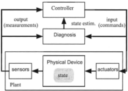
We consider a diagnosis system connected to a feedback con­ trol loop between a plant and its controller (Figure I). The inputs of the plant are the commands issued by the controller; its outputs are measurements returned back to the controller. The role of the diagnosis system is to observe the inputs and the outputs to the plant, and to report a state estimation, track­ ing the evolution of the unobservable state of the plant. This task is substantially more complex than diagnosis for a com­ binatorial, memory-less system. An estimation consists of a set of possible states of the plant, in the following referred to as a belief state. Although diagnosis might rank these states based on likelihood, as a first approach we ignore that aspect. We also disregard issues such as the correspondence between the model of the plant and the plant itself. We will focus on plants modeled as finite-state discrete systems. We assume that we have a model of the plant as a partially observable transition system, according to the following definition.

Definition 1 A (partially observable) plant is a structure (X, U, Y, 8, A), where X, U, Y are finite sets, respectively called the state space, input space and output space, o C X x U x X is the transition relation, and A C X x Y is the observation relation.

We assume that a plant P = (X, U, Y, o, A) is given. We use x, x0 , x1, ... to denote states of P, u, uo, u1 , .. . to denote inputs of P, y,yo,Yl, ... to denote outputs of P. We write x ~ x' for (x, u, x') E o, and xfy for (x, y) E A. The state is the "hidden" part of the plant: only the sequences of inputs and outputs are observable. P covers all types of behaviors that diagnosis is expected to handle - including faulty behaviors, with X containing faulty states. In general, P need not be deterministic. Thus, the state after a transition may not be uniquely determined the state before the transition and by the input. Observability is modeled by associating to each state a (non empty) set of possible outputs. It is therefore possible to model different forms of observation, e.g. when the information conveyed by the sensors is also uncertain. In this paper, we present the (input, state and output) spaces of a plant by means of assignment to (input, state and output) variables ranging over finite sets of values; the transition and observation relation can be compactly presented with boolean formulae. (Notice however that the content of the paper is independent of the specific description used to present P.)

Definition 2 A feasible execution of k :::: 0 steps in P is a sequence a= Xo,Yo,u1,X1,Y1,u2,···,uk,Xk,Yk. such that Xi-l ~ X; for 1 :::; i :::; k, and x;fy; for 0 :::; i :::; k. We define ~P as the set of all feasible execu­ tions of P . The observable trace of a feasible execution a is w = Yo, u1, Yl, .. . , uk, Yk· We write a : Xo ~ Xk. if such a a exists.

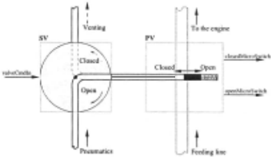
The above definition defines the dynamics of a plant and its observable counterpart. Notice that if an execution a has k steps, then the corresponding trace w E Y x (U x Y) k. The set of traces is in general a subset of Y x (U x Y) *. In the following we use a to denote a feasible execution, and w to denote the corresponding (observable) trace. For explanatory purposes, we consider the plant outlined in Figure 2, that is a simplified segment of the real-world application described in Section 6. A pneumatic valve (PV) controls the flow of a feeding line to the engine, and it is closed in its resting posi­ tion (determined by the action of a spring). A solenoid valve (SV), when open, can open PV by directing the pneumatic flow against the spring. When SV is closed, the action of the spring is no longer contrasted and PV can close. SV can re­ ceive an input (open/close), but has no observables. PV has two sensors, each providing information on a position (e.g. whether it is open or not). Both valves can become stuck in their current position. The position of the valves influ­ ences the pneumatic and engine flows. Each of the valves has two unobservable variables: state, with values open and closed, and failure mode, with values stuck and ok. The input variable can take the values no- cmd, open, and close. The effect of a command depends on the current status. Failures can occur at any time, and are permanent. Sensors of PV are also associated with a failure mode variable, that determines what information is conveyed.

3 Diagnosability

Run-time diagnosis starts from a (possibly partial) initial knowledge, observes the sequence of inputs and outputs, and tries to update a belief state that is an estimate of the possible states of the plant. For instance, if SV is commanded open, and the PV is not sensed open, then some problem should be diagnosed. It could be that SV or PV are stuck, or even that both PV sensors are not working correctly. Ideally, a diagno­ sis function should return belief states that are as specific (i.e. as small) as possible, but include the actual state of the plant.

Definition 3 A diagnosis junction for P is a function ~ : 2x x Y x (U x Y)* -+ 2 . Let x 0 C 2x. A diagnosis value x = ~(x0 , w) is correct w.r.t. x 0 and w, if and only if. for any x 0 E x 0 and x such that x 0 ~ x, we have x E x. ~ is correct if and only if ~(xo, w) is correct for any Xo and w.

The intuition behind correct diagnosis values is that they en­ compass all potential current states, so that they cannot miss the actual state. In the following, we restrict ourselves to cor­ rect diagnosis functions.

Diagnosability aims at detecting if (parts of) the hidden state can be accurately tracked by looking at the observable traces. We use diagnosis conditions to specify which infor­ mation on the state we are interested in distinguishing.

Definition 4 A diagnosis condition for a plant Pis a pair of nonempty sets of states c1, c2 C X , written c1 ..l c2.

We can express fault detection, i.e. telling if any fault is present (fault ..l ·fault), or fault separation, i.e. distin­ guishing between different faults (or fault classes) (fault a ..l faultb) . Intuitively, a diagnosis value is not satisfactory if it intersects with both sides of the condition. In the example, a fault separation condition is not satisfied if we have a be­ lief state containing both a state where PV is faulty, and one where SV is faulty.

However, it would be unrealistic to require that diagnosis pro­ vide correct and exact state estimations, instantaneously and under all circumstances. For instance, a stuck PV will stay unnoticed at least as long as SV is not operated. Rather, we require a diagnosis system to be able to decide between al­ ternative conditions on the state of the system in the context where the distinction becomes critical.

Definition 5 A diagnosis context for P is a structure C = (B, :E12 ), where B is an equivalence relation on X, and :E 12 C :Ep x :Ep. xo satisfies B (x0 ~B), i.ffxo x xo c B. (xo, w) ~ C iff Xo ~ B, and there exist ( a1, a2) E :En Xo1, Xo2 E Xo, such that a 1 : Xo1 ~ x1 and a2 : Xo2 ~ x2.

Intuitively, B defines the initial conditions under which diag­ nosability is to be investigated, by inducing of a set of disjoint belief states. Basically, the initial belief state x0 must fall within one of the belief states induced by B (the condition on B can be stated as (xol' Xo2) E B for all Xol, Xo2 E xo). For example, B can partition states according to the positions of PV and SV, to capture the assumption that we initially (only) know those positions. :E12 characterizes pairs of relevant exe­ cutions. For instance, we may want to express the fact that the controller commands SV to be open and closed at least one time. In the case of fault detection, we might want to state that the elements of :E 12 are pairs of traces, there the first are without faults, while the second ones have exactly one fault. Notice that expressing :E12 as :E1 x :E2 would be inadequate: for instance, in fault separation it would be impossible to con­ strain the two runs to have different failures. In the following we assume that a context C = (8, :E12 ) is given. The notion of diagnosability is precisely characterized as follows.

Definition 6 A diagnosis value x satisfies c1 ..l c2, written x F c1 ..l c2, if and only if either x n c1 = 0 or x n c2 = 0. A diagnosis function ~satisfies c1 ..l c2 over C, written ~,C ~ c1 ..l c2, ifandonlyif.forall(xo,w) ~ C, we have ~(xo,w) ~ c1 ..l c2. A condition c1 ..l c2 is diagnosable in P over C if and only if there exists a correct diagnosis function that satisfies it.

4 Diagnosability as Coupled Reachability

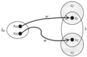
Our approach to reasoning about diagnosability is based on refutation, i.e. we search for ways in which the diagnosability property can be violated. Intuitively, we verify the diagnos­ ability of c1 ..l c2 by checking that P does not have a critical pair, i.e. two executions with identical observable traces, one leading to c1 , one leading to c2 (see Figure 3).

Definition 7 A critical pair of a plant P, with trace w, for a diagnosis condition c1 ..l c2, is a pair of feasible executions w d w . I a1 : Xo1 --+ X1 an a2 : xo2 --+ X2, wntten a1 a2 : Xo1Jxo2 ~ x1Jx2, such that X1 E c1 and X2 E C2 . The critical pair a 1Ja2 is covered by a diagnosis context C = (B, :E12), ijf(xo1, Xo2) E B, (a1, a2) E :E12·

The absence of critical pairs for c1 ..l c2 in a given context is a necessary and sufficient condition for c1 ..l c2 to be diag­ nosable in that context.

Theorem 8 c1 ..l c2 is diagnosable over C in P, if and only if P has no critical pair for c1 ..l c2 in C.

To prove the theorem, we introduce the notion of perfect di­ agnosis, written ~, i.e. the most specific correct diagnosis function that can be made assuming full knowledge of P.

Definition 9 The perfect diagnosis for a plant P is the diag­ nosis function ~(xo,w) = {x l3xo E xo.xo ~ x}.

Given an initial belief state xo and trace w, ~(x0 , w) returns exactly all states that can be reached from x0 through w. It is easy to see that ~ is correct, and that it is the most informative diagnosis function, i.e. ~ ( x 0 , w) C ~ ( x0 , w) for any correct ~ . We observe that a condition c1 ..l c2 is diagnosable in a plant P over a context C if and only if~' C ~ c1 ..l c2 : from Definition 6, if X c x' and X 1 F Ct ..l C2, then X ~ Ct ..l c2. Therefore, ~ satisfies any diagnosable condition, since its diagnosis values are more specific than any other correct diagnosis function.

Proof of Theorem 8 c1 ..l c2 is not diagnosable in P over C; if and only if there exist x o and w such that ~ ( x0 , w), C ~

c1 .l c2; if and only if there exist (a1,a2) E ~12 and Xot, xo2 E io such that a1 : Xot ~ Xt and a2 : xo2 ~ x2 ; if and only if there exists a critical pair for a1 la2 for Ct .l c2 in C. Q.E.D.

In order to search for critical pairs in P, we build the cou­ pled twin plant for P, written P · P, i.e. a "Siamese twins" plant, made out of two copies of P, whose inputs and outputs are forced to be identical.

Definition 10 The coupled twin plant of Pis the plant p.p = (X·X, U, Y,o·o, A· A), where X ·X c X 2 , and,forall Xt,X2 EX, (x1,x2) EX ·X iffthereexistsy E Y such that (xt,Y) E Aand(x2,y) E A; ((xt,x2),u,(xi,xm Eo ·o iff (xt,u,xi) E cSand(x2,u,x~) E c5,· ((x1,x2),y) E A·Aif! (xt , y) E A and (x2, y) E A.

In the following, we assume that the coupled twin plant P · P of Pis given. The importance of the coupled twin plant construction is shown by the following theorem.

Theorem 11 a1 : Xot ~ Xt and a2 : Xo2 ~ x2 are two feasible executions in P if and only if a12 : (Xot, Xo2) ~ (xt, x2) is a feasible execution in P · P .

This is easily demonstrated by induction on the length k of executions. When k = 0, then w = YO· From Defini­ tion 10, xot/Yo and xo2/Yo iff (xot, xo2) E X · X and ((xot,Xo2),yo) E A· A. The step case is proved by extend­ ing with a transition the executions oflength k, for which the theorem holds. From Definition 10, the transitions in P · P mimic the transitions in P. For the last observation, we rea­ son as for the base case.

5 Diagnosability via Model Checking

We work in the framework ofModel Checking [Clarke et al., 1999], a formal verification technique that is increasingly ap­ plied to the design of industrial digital systems (e.g. com­ munication protocols, hardware design). Model checking al­ lows to verify if the (possibly infinite) behaviors of a system satisfy a given property. The system being analyzed is pre­ sented as a Kripke structure, while properties are expressed in a temporal logic [Emerson, 1990]. Model checking algo­ rithms are based on the exhaustive exploration of the Kripke structure. The technique is completely automatic and, if a property is violated, it can produce a counterexample, i.e. a simulation witnessing the violation. Symbolic model check­ ing [McMillan, 1993] is based on the manipulation of sets of states described by boolean formulae; efficient engines, such as Binary Decision Diagrams (BDDs) [Bryant, 1986] and SAT solvers [Moskewicz eta!., 2001 ], provide a basis for efficient representation and exploration of the search space.

Our approach to diagnosability inherits several elements from model checking. The first is that a plant P can be asso­ ciated with a Kripke structure K p representing its behavior. This makes it possible for us to directly analyze a plant with model checking techniques. A Kripke structure is basically a nondeterministic transition system, where transitions are not labeled, while information is associated with states (i.e. each state is associated with a valuation to the state variables of the structure). The mapping from plant to Kripke structure is rather simple, and is based on the idea that the state, input and output spaces of the plant can be encoded into the state space of the Kripke structure. The information on the inputs, labeling the transitions in P, simply becomes part of the state of Kp, and is to be interpreted as "the input that will be pro­ cessed in the next transition". More formally, each states in Kp is associated with a valuation that characterizes a triple xfy ~. i.e. P is in state x , output y is observed and input u is received. The dynamics of P directly induce the dynam­ ics of Kp . For each feasible execution u in P of the form xo, Yo, Ut, Xt, Yt, u2, .. . , uk, Xk, Yk there is a corresponding path 1r in Kp , i.e. a sequence of states s0 , s1 , .. . Sk where each Si is associated with the triple xdyi ~- The same mapping lifts to the coupled twin plant construction. (In the above description, we omit a few technical details, having to do in particular with the fact that a Kripke structure is as­ sumed to be total, i.e. every state has at least one successor. In this way, it is possible to assume that the analyzed paths are infinite. Since inputs become part of the state, it is possible that the transition relation is no longer total. There are stan­ dard workarounds to this problem, routinely used in verifica­ tion and in AI planning. See for instance [ Cimatti and Roveri, 2000] .) In the following, we assume that Kripke structure Kp.p corresponding to the coupled twin plant P ·Pis given.

The second element from model checking is the symbolic representation. The state of K p.p is defined with a vec­ tor of variables (xt, x 2 , u , y), respectively ranging over X , X, U and Y. We can use formulae to characterize sets of states. In Kp.p we express atomic propositions over such variables. We can have equalities between variables and the corresponding values: Pl . PV. input = close denotes the set of states where the first instance of PV receives the close command. Variables of the same type can be equated: Pl. SV. failure mode= P2 . SV. failure mode de­ scribes the set of states where the two instances of SV in the twin plant have the same failure mode. Any subset c of X x X x U x Y can be described with a formula c(x1,x2,y, u) . For instance, the formula c1(x1) 1\ c2(x2) expresses a state of the twin plant where the first instance is in c1 and the second is in c2. Similarly, B(x1, x2) is a (proposi­ tional) formula expressing, in symbolic form, the equivalence relation (}.

The third ingredient from model checking is the use of temporal logics to characterize behaviors of the system over time. We use LTL (Linear Temporal Logic [Emerson, 1990 ]), where formulae are constructed starting by combining atomic propositions with boolean operators and temporal modalities. If¢ and 1/J are LTL formulae, so are F ¢ (sometimes in the future¢), G ¢(always in the future ¢), 1/J U ¢(sometimes in the future¢ and, until then, 1/J), X¢ (in the next time step¢). An LTL formula¢ holds on a path 1r (written 1r f= ¢),iff¢ is true in 1r at (step) 0 (written 1r 0 f= ¢). Ifp is an atomic propo­ sition, then 1ri f= p iff p is true according to the assignment associated with the i-th state of 1r. Boolean connectives have the standard interpretation (e.g. 1ri f= ¢ 1\ 1/J iff 1ri f= ¢and 1ri f= 1/J ). The interesting cases of temporal operators are as follows. 1ri f= F ¢ iff there exists j 2: i such that 1rj f= ¢. 1ri f= G ¢ iff for all j 2: i 1rj f= ¢. 1ri f= 1/J U ¢ iff there exists

MODULE SV_type (cmd_in) MODULE PV type ( ) VAR pneumaticsLinein : {abvThresh,blwThresh}; VAR valvePositionValue : {open,closed}; VAR mode : {stuckOpen,nominal,stuckClosed}; DEFINE _faultmodes := {stuckOpen,stuckClosed}; DEFINE broken := mode in faultmodes; DEFINE brokencount := _broken; DEFINE _brokenprob := case mode mode else esac; stuckOpen stuckClosed 3; 3; 0; MODULE EX_type (sv_cmd_in, . .. ) sv : SV_type(sv_cmd_in); PV : PV_type( ) ; DEFINE brokencount . - SV. broken + PV. broken +

j ;::: i such that 1rj f= ¢and, for all i :::; h < j, 1rh f= '1/;. 1ri f= X¢ iff 1ri+ 1 f= ¢. An (existential) model checking problem K f= ¢, read¢ (existentially) holds inK, amounts to detecting if K admits a path where ¢ holds.

A diagnosis condition with a context is represented with temporal logic formula ¢ such that K p .p f= ¢ holds iff there is a critical pair. We express reachability in P · P of a criti­ cal pair for a diagnosis condition c1 j_ c2 with the formula: F (c1(x1) 1\ c2(x2)). Model checking can be run on the problem Kp.p f= F (c1(x1) 1\ c2(x2)) . Ifthe answer is true, then we have a witness for the a critical pair. Given the con­ text C = (B, E12), we enforce the initial condition() with the formula B(xt,x2) 1\ F (c1(x1) 1\ c2(x2)). The conjunc­ tion has the effect of restricting the analysis to the paths in Kp.p starting from the states that satisfy B. E12 is taken into account assuming that a characterization of the sets of traces is described by an LTL formula E 12 (x1, X2Y, u). The model checking problem corresponding to diagnosability is Kp.p f= B(x1, x2)/\E12 (x1, x2y, u)/\F (c1 (x1) 1\ c2(x2) ). In practice, several simplifications are possible. Often E12(xt,x2, u,y) can be expressed in terms ofpropositional constraints ¢ 12 (x1, x2, u , y ), that must hold on all the states of the execution; in such cases diagnosability in context C is basically represented by the LTL formula B(x1, x2) 1\ (¢12(Xt,X2, u,y) U (c1(x1) 1\ c2(x2))) . Notice that the formula holds if the path condition ¢ 12 holds until the con­ ditions c1 and c2 are reached. When the context does not constraint the executions, the above formula is equivalent to B(x1 , x2) 1\ F (c1 (xi) 1\ c2 (x2) ).

MODULE main VAR sv_cmd : { no_cmd, open, close }; Pl : EX_type(sv_cmd, . .. ) ; P2 : EX_type(sv_cmd, . . . ) ; INVAR (Pl.PV.sense_open = P2.PV.sense_open) &

6 Experimental Evaluation

We analyzed the practical applicability of our approach within the Livingstone framework. Livingstone is a model­ based health monitoring system developed at NASA Ames [Williams and Nayak, 1996]. It uses a model of a physical system, such as a spacecraft, to infer its state and diagnose faults from observations. Livingstone is one of the three parts of the Remote Agent (RA), an autonomous spacecraft con­ troller developed by NASA Ames Research Center jointly with the Jet Propulsion Laboratory. RA was the first AI software to control an operational spacecraft [Muscettola et a!., 1998]. Livingstone has also been used in other applica­ tions such as the control of the In-Situ Propellant Production system (ISPP) for Mars missions [Clancy eta!., 1999], the monitoring of a mobile robot [Simmons eta!., 2001], and In­ telligent Vehicle Health Management (IVHM) for experimen­ tal space transportation vehicles [Bajwa and Sweet, 2002].

Livingstone uses a qualitative relational model describing the evolution of observable and hidden variables. Continuous physical domains are abstracted into discrete intervals such as {low, nominal, high}. Each component has a mode variable identifying its nominal and fault modes. Livingstone models are specified in a hierarchical, declarative formalism called JMPL, or using a graphical development environment. Livingstone observes the commands issued to the plant and uses the model to predict the plant state. It then compares the predicted state against observations received from the actual sensors. If a discrepancy is found, Livingstone performs a diagnosis by searching for the most likely configuration of component modes that are consistent with the observations.

Livingstone models directly induce a synchronous transi­ tions systems, very similar to a plant model. Pecheur and Simmons [Pecheur and Simmons, 2000] have developed a translator able to convert a Livingstone model and a re­ lated set of specifications in the language of the SMV model checker [McMillan, 1993 ], and to convert back the diagnostic traces in terms of the Livingstone model. Figure 4 outlines the structure of the example plant in SMV language. For each component type, there is a corresponding module. The first module statements define the model for the SV and the PV. For each of the components, a set of variables is defined, the dynamics of which is directly induced from the Livingstone model. Notice the _ brokenprob variable, whose numeri­ cal value is the (negated) logarithm of the probability of fail­ ure for the component (e.g. 10 - 3 ). This enables for a (rough) analysis of failure probabilities. These modules are instan­ tiated in the EX module, with a parameter representing the commands to PV.

In order to tackle diagnosability, we devised a systematic way of constructing the SMV coupled twin plant of a Living­ stone model. The construction is outlined in Figure 5. The EX plant is instantiated twice in the main, at top level, gen­ erating Pl and P2 . The same input variable (sv _ cmd) is given in input to both instances. Then, the outputs of the two instances of the plant are constrained to exhibit the same behavior by means of an INVAR statement, i.e. a condition that must hold in all states. The SMV language enables for the specification of context. The basic building blocks of the properties are propositional conditions over states, that can be expressed by means of the DEFINE construct. For in­ stance, it is possible to express conditions on the number of failures, using the _brokencount variable defined in Fig­ ure 4. For instance, Pl . brokencount < 2 in the main module states that at most one failure can occur in the first instance of the circuit.

In the experimental analysis, we tackled several problems for the Livingstone model of the Main Propulsion System for the X-34, a next-generation vehicle for the Space Shut­ tle [Bajwa and Sweet, 2002]. We interacted with the NASA experts of diagnosis, to check the representational adequacy of our formalism, and to characterize diagnosability problems of practical relevance. The problems were defined starting from simulation runs, that tested a specific fault in a specific context. We remark the impact of our approach is far be­ yond the one of testing, since it performs an exhaustive anal­ ysis (though at a higher abstraction level) within the cases captured by the context. The experimental evaluation was carried out by running different symbolic model checking tools on models described in SMV language, such as the CMU SMV [McMillan, 1993], Bwolen Yang's version of SMV [Yang eta!. , 1999], and NuSMV [Cimatti eta/., 2002]. While the former ones are based on Binary Decision Dia­ grams (BDDs) [Bryant, 1986], NuSMV also enables the use of SAT-based techniques [Moskewicz eta!., 2001]. This ac­ tivity suggested several considerations. First, the experimen­ tal analysis was fundamental to tune the formalism. Several improvements (e.g. the notion of context) were conceived while trying to encompass representational issues arising in practice. Second, contexts are incrementally characterized. Although the requirements for the diagnosis system can usu­ ally suggest an initial version for the context, it is seldom the case that the precise conditions for diagnosability are known (or can be precisely stated) in advance. The ability of the model checker to find critical pairs was very useful in the re­ finement, since it helped to explain why diagnosability fails, i.e. to understand whether the context is not strict enough, or because a problem was found.

In terms of performance, the critical factor was the size of the models to be analyzed. The most significant plant we analyzed has about 800 scalar variables. This number almost doubles in the case of the twin plant, and (after the elimination of equivalent variables) we are left with mod­ els having about 600 state variables. Different versions of SMV were used to tackle the resulting diagnosability prob­ lems. All the BDD-based verification engines were defeated by the size of models for coupled twin plants (i.e. no solution found after running for 24hs). This failure occurred despite the use of advanced techniques such as dynamic reordering, invariant discovery, and conjunctive partitioning. We remark that some of these BDD-based engines, most notably Bwolen Yang's SMV, were able to tackle verification problems on single plants very efficiently. On the other hand, the use of model checking techniques based on SAT solving, imple­ mented in the NuSMV system [Cimatti et al., 2002], proved to be very effective on these problems. We used a combined approach, integrating bounded model checking (oriented to finding bugs) and inductive reasoning. The SAT-based engine of NuSMV was able to solve all the verification problems in less than two seconds. The analysis of the results shows that Livingstone models tend to feature a huge state space but little depth; therefore, the symbolic processing provided by SAT turns out to be very appropriate. It is worth mention­ ing that, while trying to refine a diagnosability property, we discovered an unexpected behavior in the model of the X-34. Further analysis highlighted a missing statement in the de­ scription. This result is quite significant, since the model had been repeatedly tested.

7 Related Work

The idea of diagnosability has received a lot of attention in the framework of Discrete Event Systems. In [Sampath et al., 1995; 1996], diagnosability is precisely defined and an algorithm for checking diagnosability is presented. The ap­ proach is limited to failures represented as reachability prop­ erties. Jiang and Kumar [Jiang and Kumar, 2002] generalize the approach to the case of failures described as formulae in linear temporal logics. The approach is based on a polyno­ mial algorithm for testing the diagnosability, formulated with techniques from automata theory [Jiang et al., 2001]. In par­ ticular, they define a self-product automaton similar to our twin plant. Console, Picardi and Ribaudo [Console et a/., 2000] propose the use of a particular form of process alge­ bras, PEPA, for the formalization and the analysis of diagno­ sis and diagnosability problems.

Our work is rather different from the works mentioned above, that are mostly oriented to the definition of the theoret­ ical framework, and do not address the problems related to the practical application of the proposed techniques. Our objec­ tive is the definition of an effective platform for the analysis of diagnosability, that can be practically applied in the de­ velopment process of diagnosis systems. The "twin-models" approach allows us to directly reuse standard model check­ ing tools, without having to reimplement a complex tableau construction described in [Jiang et al., 2001]. Furthermore, our approach preserves the semantics of the problem, thus making it possible to tune the decision procedure to the ap­ plication domain. In terms of expressivity, our work shares several underlying assumptions with [Sampath et al. , 1995; 1996], considering failures that can be represented as reach­ ability conditions. Compared to [Jiang et al., 2001], we only tackle zero-delay diagnosability, although it seems that our framework could be extended in this respect.

Our approach makes no hypothesis on the way the con­ troller exploits the information provided by the diagnosis sys­ tem. For this reason, we introduce the notion of context in order to qualify the conditions under which diagnosability should hold. In active diagnosis [Sampath eta!., 1998], the controller is designed taking into account the issues of di­ agnosability. Similar problems are also tackled in planning under partial observability, where the planner can decide the most appropriate actions to diagnose the fault, e.g. by probing the system with actions that will provide suitable information, and recover from it (see for instance [Bertoli eta!., 2002]).

8 Conclusions

In this paper, we have proposed a novel approach to the ver­ ification of diagnosability, with emphasis on its practical ap­ plicability. Our work is based on a new conceptualization of the problem, with the twin plant construction and the use of temporal logic formulae to describe the context of a diagnos­ ability problem. To the best of our knowledge, this is the first approach to diagnosability that enables the direct exploitation of symbolic model checking technology. We tackled signif­ icant diagnosability problems from a real-world application, discussed a practical methodology for the incremental refine­ ment of diagnosis contexts, and were able to verify large­ sized problems. In the future, we will try to take into account the fact that diagnosis can propose several candidates, with different degrees of likelihood. A compositional approach to verification, exploiting the modular structure of the design, will be investigated. In the longer term, we plan to tightly in­ tegrate the approach within the Livingston toolset, in order to allow Livingstone application developers to use model check­ ing to assist them in designing and correcting their models, as part of their usual development environment.