A flexible and robust similarity measure based on contextual probability

1 Introduction

Natural and artificial intelligent agents rely on different inference and reasoning strategies to achieve their goals and maintain their intended behavior. Arguably, two of the more successful strategies are based on the notions of analogy 1

∗Also LITA, Université de Metz, Ile du Saulcy, 57045 Metz Cedex, France.

1 Here we consider the subject of analogy in the following, relatively narrow, sense: objects are represented by feature vectors rather than the typical graphs; we do not consider transfer of knowledge from one object to another; we do not consider cross-domain knowledge but assume all objects share common set of attributes.

Werner Dubitzky

School of Biomedical Science University of Ulster at Coleraine Northern Ireland w.dubitzky@ulster.ac.uk

and similarity. This is evidenced by the large volume of AI research in the areas of analogical reasoning and case-based reasoning [Vosniadou and Ortony, 1989; Kolodner, 1993]. In the context of available background knowledge, analogy can be viewed as a logical inference process [Davies and Russell, 1987]. Another way of looking at analogy holds that similarity can provide a probabilistic basis for inference, and that a quantitative framework can be developed for the probability that an analogy is correct as a function of the degree of similarity measured or observed [Russell, 1986]. This study is concerned with the latter view of modeling analogy.

Distance measures (or, equivalently, similarity measures) are central to many areas related to AI, including reasoning under uncertainty, knowledge-based systems, machine learning, pattern recognition, data mining, analogical, case-based, instance-based reasoning, and to other fields such as statistics, operations research and decision theory. A large number of distance metrics and measures are available and a particular choice may have considerable implications for the success of the problem that is to be addressed.

Distance functions are broadly categorized into those that can handle ordinal input data, nominal input data, and heterogeneous input data, consisting of both ordinal and nominal data 2 . Ordinal distance functions make use of the intrinsic total ordering relation in the underlying attribute values, which are either continuous (e.g. weight of an object) or discrete (e.g. number of obstacles). A nominal or symbolic attribute is a discrete attribute whose values do not necessarily exhibit a total order relation. For example, an attribute representing the role of crew member may have the values scientist, mission specialist and commander. Using an ordinal distance measurement on such values is meaningless.

Because the notion of 'distance' is intrinsically numerical, most available distance measures are defined for data with ordinal attributes. However, distance measures that can process nominal attributes are required by many modern AI algorithms. Some measures that handle nominal attributes do exist. The most well known measure of this kind is the Value DifferenceMetric (VDM) [Stanfill andWaltz, 1986]. It is defined in terms of attribute values that are conditioned by posterior probabilities of a class. Hence, like some other distance measures, the VDM is restricted to classification tasks.

2 Here we consider two scales of measurement: ordinal and nominal. In an ordinal scale, values (discrete or continuous) are ordered whereas in a nominal scale, (discrete) values are unordered.

To cope with heterogeneous data, containing both nominal and ordinal attributes, two approaches are commonly taken: (1) The data is transformed into one of the two data types that complies with the distance measure used, and (2) two types of distance measures are combined and handle the data separately in accordance with the data type (see, for example, [Wilson and Martinez, 1997]). However, both approaches are problematic when it comes to the interpretation of the results.

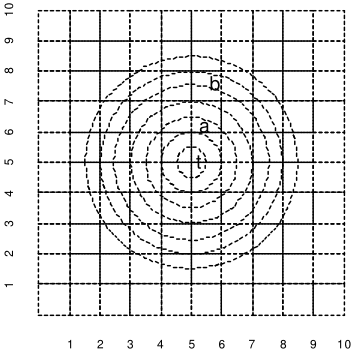
The novel distance measure proposed in this study is called Neighborhood Counting Metric (NCM). It is derived from a probability function and it can handle both nominal and ordinal attributes in a conceptually uniform way. Intuitively, it can be understood or interpreted as follows (see Figure 1): If we consider all neighborhoods, N, around a data point, t, then those data points closer to t should be included in more of these neighborhoods, N, than points that are not close to t. Usually neighborhoods are interpreted in terms of distance. However, if we adopted this interpretation, we would define one distance function in terms of another. To avoid this dilemma, we interpret neighborhood without distance through the concept of hypertuples [Wang et al., 1999] for both nominal and ordinal attributes. As a result, our distance measure applies to both ordinal and nominal attributes in a uniform way.

The new NCM is conceptually simple, it is straightforward to implement, and it has the added property that it is independent of the underlying analytical or reasoning task (e.g. classification). The measure's clear and unambiguous meaning is defined by the number of neighborhoods of a query that include or cover a given data point.

Paper outline: Section 2 presents a short review of distance measures relevant to this study; it is followed by Sections 3 and 4, which present mathematical details of the new similarity measure. In Section 5 the empirical evaluation of the method is presented and its results discussed. The paper concludes with a summary and a brief discussion of future work.

2 A brief review of important distance functions

Two of the most common distance functions are Euclidean distance and the Hamming distance. The former is restricted to ordinal and the latter is usually used for nominal attributes. The Heterogeneous Euclidean-Overlap Metric (HEOM) [Wilson and Martinez, 1997] combines the Hamming and the normalized Euclidean distance functions and can therefore be used on heterogeneous data.

The Value Difference Metric (VDM) [Stanfill and Waltz, 1986] is designed to handle nominal attributes in classification tasks only. It uses pre-computed statistical properties from available training data and can be interpreted in terms of probabilities. The Heterogeneous Value Difference Metric (HVDM) [Wilson and Martinez, 1997] combines the Euclidean distance and the VDM. It is therefore able to handle heterogeneous data, but because of its VDM heritage it is confined to classification tasks.

The Interpolated Value Difference Metric (IVDM) [Wilson and Martinez, 1997] extends the VDM to scenarios involving ordinal attributes. In the learning phase, it employs a discretization step to collect statistics and determine the probability for the discretized values (Pa,x,c in the VDM formula), but then retains the continuous values in the training data for later use in the application or testing phase. The IVDM requires a non-parametric probability density estimation to determine the probability values for each class. The Discretized Value Difference Metric (DVDM) is the same as the IVDM except that it avoids the retention of the original continuous values but uses only the discretized values.

[Blanzieri and Ricci, 1999] introduced the Minimal Risk Metric (MRM), a probability-based distance measure for classification and case-based reasoning. It minimizes the risk of misclassification and depends on probability estimation techniques. As a result, the MRM exhibits a high computational complexity and is task-dependent.

3 A probability function

Let V be a (non-empty) universe of discourse. A S-field F on V is a collection of subsets of V, such that:

1. V ∈F ;
2. If A∈F then A′ ∈F , where A′ is the complement of A;

A probability function P over V is a mapping from F to [0,1] satisfying the three axioms of probability [Ash, 1972]. If P is restricted to V, it is called a probability mass function (discrete) or probability density function (continuous).

Suppose we have a probability function P as defined above. For X ∈F let f (X) be a non-negativemeasure of X satisfying f (X1 ∪X2) = f (X1)+ f (X2) if X1 ∩X2 = /0. As an example, we can take f (X) for the cardinality of X.

Consider a function G : F → [0, 1] such that, for X ∈ F ,

where K = �E∈F P(E) f (E). It can be easily shown that G is a probability function.

G(X) is calculated from all those E ∈ F that overlap with X (i.e., f (X ∩E) ̸= 0). These E's are relevant to X and serve as the contexts in which G(X) is induced. Each such E is called a neighborhood of X. In other words a neighborhood of X is an element E of F , i.e., a subset of V, such that E overlaps X.

In practice P is usually not known, but a sample of data drawn from the data space according to P is commonly available. P can be estimated from the sample by either parametric or non-parametric techniques. In some tasks (e.g., classification) the point-wise probability is needed. When there is insufficient data, which is not uncommon, the point-wise probability may be difficult to estimate using non-parametric methods. However, it is likely that probability can be estimated for some regions (contexts) in the data space based on the sample. Using the G probability function, we can estimate the G probability for any single data point from knowledge of the P probabilities of various regions or contexts. This provides us with a formal way of inference about probability under incomplete (hence uncertain) situations.

To calculate the G probability for X ∈ F in practice, we need to

1. Find the set of all neighborhoods appropriate to the problem at hand,
2. Estimate the P probability for every neighborhood,
3. Finally, estimate (calculate) the G probability for X according to its definition.

In classification tasks, we can further calculate the conditional G probability of a class given a single data point in a similar fashion. While this may appear to be computationally expensive, it is often possible to derive a simple formula for G.

Depending on what F is and how neighborhoods are defined, we can use the G probability for different tasks. In Section 4 we take F to be the set of all regions in a multidimensional space definable as hypertuples and our similarity measure is derived from this interpretation.

3.1 Estimation of G

This section describes how G is estimated for a data point from data samples. Let D be a sample of data drawn from V according to an unknown probability distribution P. Our aim is to calculate ˆG(t|D) for any t ∈V.

To calculate G we need P, which can be estimated from data assuming the principle of indifference as follows: For any E ∈ F ,

where |E| is the number of elements in E and n is the number of elements in D. Additionally we assume that f (X) = |X| for X ∈ F .

We then have,

where K is a normalisation factor, and cov(t, x) is the number of such E ∈ F that covers both t and x. We call this number the cover of x with respect to t.

To obtain cov(t,x), a straightforward approach would be to iterate over all E ∈ F and check if E covers both t and x. Clearly, such a process is undesirable because of its exponential complexity. In Section 4 we will present an efficient way of calculating cov(t,x).

4 Measuring distance through counting

This section considers an interpretation of neighborhood and derives a formula for calculating cov(t , x), which is then taken as a measure of similarity or distance.

4.1 Neighborhood

Pursuing a non-distance-based conceptualization of neighborhood, we interpret a neighborhood as a hypertuple [Wang et al., 1999], and a neighbor as a data point (or tuple) covered by some neighborhood. So a neighborhood of a tuple is a hypertuple that covers the tuple.

Hypertuples

Let R = {a1,a2, · · · ,an} be a set of attributes, and dom(a) be the domain of attribute a ∈ R. Furthermore let V def = � n i=1 dom(ai) and L def = � n i=1 2 dom(ai) . V is the data space defined by R, and L an extended data space. A (given) data set is D⊆V - a sample of V.

The attributes can be either ordinal or nominal. For simplicity, we assume the domain of any attribute is finite, but the results are not limited to finite domains.

If we write an element t ∈V by 〈v1,v2, · · · ,vn〉 then vi ∈ dom(ai). If we write h ∈ L by 〈s1, s2, · · · , sn〉 then si ∈ 2 dom(ai) or si ⊆ dom(ai).

An element of L is called a hypertuple, and an element of V a simple tuple. The difference between the two is that a field within a simple tuple is a value while a field within a hypertuple is a set. If we interpret vi ∈ dom(ai) as a singleton set {vi}, then a simple tuple is a special hypertuple. Thus we can embed V into L, so V ⊆ L.

Consider two hypertuples h1 and h2, where h1 = 〈s11,s12, · · · ,s1n〉 and h2 = 〈s21,s22, · · · ,s2n〉. We say h1 is covered by h2 (or h2 covers h1), written h1 ≤ h2, if for i ∈ {1, 2, · · · , n},

Furthermore the sum of h1 and h2, written by h1 +h2 def = 〈s1,s2, · · · ,sn〉, is: for each i ∈ {1,2, · · · ,n},

The product operation ∗ can be similarly defined. It turns out that 〈L,≤,+,∗〉 is a lattice.

For a simple tuple t, t(ai) represents the projection of t onto attribute ai. For a hypertuple h, h(ai) is similarly defined.

A hypertuple can be generated by taking one subset from each attribute. Let ai be an attribute, i = 1,2, · · · ,n; Si be the set of all subsets of the domain of ai; and N′′ i def = |Si|. Then a hypertuple h is an element of �i Si. Therefore the number of all hypertuples is �i N′′ i .

If ai is nominal, then Si = 2 dom(ai) and so N′′ i =2 mi , where mi = |dom(ai)|. If ai is ordinal, then an element s ∈ Si corresponds to an interval [min(s),max(s)]. As a result, some elements of Si may correspond to the same interval, and hence become equivalent. In general we have the following number of distinctive intervals for an ordinal attribute: N′′ i =� mi-1 j=0 (mi - j) =� mi j=1 j = mi(mi+1) 2 .

Neighborhoods as hypertuples

For any simple tuple t, a neighborhood of t is taken to be a hypertuple h such that t ≤ h; and a neighbor of t with respect to h is x ∈V such that x ≤ h. By this definition any simple tuple has a neighborhood. At least the maximal hypertuple in the extended data space is a neighborhood of any simple tuple since the maximal hypertuple covers all simple tuples.

For a query t ∈V, not all hypertuples in �i Si are neighborhoods of t. For a hypertuple h to be a neighborhood of t we must have t(ai) ∈ h(ai) for all i. Therefore, to generate a neighborhood of t, we can take an si ∈ Si such that t(ai) ∈ si for all i, resulting in a hypertuple 〈s1,s2, · · · ,sn〉. If ai is nominal, the number of si ∈ Si such that t(ai) ∈ si is N′ i =� mi-1 i=0 (mi-1 i ) = 2 mi-1 since si is any subset of dom(ai) that is the super set of t(ai). If ai is ordinal, this number is N′ i = (max(ai)-t(ai)+1)×(t(ai)-min(ai)+1) since (max(ai)-t(ai)+1) is the number of ordinal values above t(ai), and (t(ai)-min(ai)+1) is such a number below t(ai). Any pair of values from the two parts respectively forms an interval.

To summarize, the number of neighborhoods of t is �i N′ i , where

(1)

Cover of simple tuples

Under the above interpretation of neighborhood, we know exactly the number of all neighborhoods of a given simple tuple t. Here we present an efficient way of calculating cov(t,x), the number of neighborhoods of t that cover x, which is needed in Section 3.1.

Consider two simple tuples t = 〈t1,t2, · · · ,tn〉 and x = 〈x1,x2, · · · ,xn〉. A neighborhood h of t covers t by definition, i.e., t ≤ h. What we need to do is to check if h covers x as well. In other words, we want to find all hypertuples that cover both t and x.

Eq.1 specifies the number of all simple tuples that cover t only. We take a similar approach here by looking at each attribute and explore the number of subsets that can be used to generate a hypertuple covering both t and x. Multiplying these numbers across all attributes gives rise to the number we require.

Consider attribute ai. If ai is ordinal, then the number of intervals that can be used to generate a hypertuple covering both xi and ti is as follows:

If ai is nominal, the number of subsets for the same purpose is:

Recall that mi = |dom(ai)|.

To summarize, the number of neighborhoods of t covering x is cov(t , x) = �i Ni, where

(2)

4.2 Use of cover as similarity measure

We use cov(t,x) as a measure of similarity between t and x, which we call the Neighborhood Counting Metric or simply NCM. That is, for any two tuples x and y, the NCM between them is

where n is the number of attributes and Ni is given by Eq.2. It is clear that NCM(x,y) ≥ 0, NCM(x,x) ≥ NCM(x,y) and NCM(x, y) = NCM(y, x). Therefore the NCM is reflexive and symmetric, the properties generally required for a similarity measure [Osborne and Bridge, 1997].

This measure can be interpreted intuitively as follows. If we consider all neighborhoods around a data tuple, those tuples closer to this tuple should be included in more neighborhoods and those farther away should be included in fewer neighborhoods (see Figure 1). As a result, closer tuples should be assigned higher cover values.

In contrast to its usual interpretation in terms of distance, we interpret the notion of a neighborhood without distance through the concept of hypertuples for both nominal and ordinal attributes. As a consequence, our novel distance measure applies to both ordinal and nominal attributes in a conceptually uniform way.

Incidentally, the NCM intrinsically handles missing values in a fashion consistent with other measures. Recall, that the NCM is a product of all Ni's, where i is attribute index. For two data tuples, t and x, if there is a missing value in t or x for attribute i, then Ni is set to 1. As a result, this attribute does not contribute towards the NCM value.

5 Evaluation

The new Neighborhood Counting Metric is task-independent and can therefore be used for classification, clustering and other analytical tasks involving distances or similarities. We empirically evaluated the NCM in the context of a classification task, using the k-nearest neighbor (k-NN) classification algorithm with and without distance-based (neighbor)

weighting [Baily and Jain, 1978]. The purpose of the evaluation is to compare the new measure with some of the commonly used distance measures in a setup involving heterogeneous data. The evaluation uses public benchmark data sets from UC Irvine Machine Learning Repository, which were selected with respect to their balance of ordinal and nominal attributes.

We implemented a k-NN algorithm with the novel NCM as well as the measures HEOM, HVDM, IVDM, and DVDM. The computational runtimes of the MRM turned out too excessive, so it was excluded from the study. In the experiments k was set to 1,6,11,16,21,16,31 and to 'MaxK' (i.e., k = the number of data tuples in the training data). We adopted a 10-fold cross-validation procedure, and for each measure and each k value we ran the cross-validation 10 times and recorded the results for subsequent analysis.

Due to space limitations, we report only some of the results in detail. Table 1 shows the results when weighting was used and k = MaxK.

A statistical significance analysis was carried out using the Student t-test (two samples, assuming unequal variances) with a = 0.05 (at a 95% confidence level). For each data set, each measure and each k value, we ran a 10-fold crossvalidation using k-NN 10 times with random partitioning of data, resulting in a sample of 10 values. For a pair of samples, by two different measures, we have a total of 20 values. So the critical value is 2.1. We then calculate the 't' values. If t ≥ 2.1 or t ≤-2.1 the two samples are significantly different (the classification rate of one sample is significantly higher or lower than that of the other). Notice that every value in Table 1 is the average of a sample of 10 values.

From Table 1 we can see that based on our experimental design the NCM achieved 17 out of 20 'significantly' higher classification success rates compared to the other methods (last row in table). Looking at the subtotals for 'nominal', 'ordinal' and 'mixture' categories (reflected by subtotals from top to bottom), the NCM achieves the largest margin over its competitors for the 'nominal' data sets, followed by 'mixture' and then 'ordinal'. This suggests that, when all data tuples are taken into consideration, the NCM is clearly superior under all circumstances.

The details of the results involving other values for k are not shown. In terms of k-changes, we observe that without weighting there was no significant difference between the used measures. When weighting was used, there was still little difference for small k values. The general trend for all measures was: as k got larger the classification success rate increased slightly but soon started to decline. The difference then showed up as the NCM displayed a much slower rate of decline and, after k > 11, the NCM consistently outperformed the other four measures (see k =MaxK as discussed above). We can conclude that the NCM produces less variable or more robust results than the other four measures.

6 Conclusion

Starting from a probability function, we have developed a novel similarity or distance measure, the Neighborhood Counting Metric, which can be used with ordinal, nominal and heterogeneous attributes in a conceptually uniform way. This measure is defined without reference to any particular analytical task (e.g., classification). This means that the measure is potentially useful for many reasoning, inferential and reasoning tasks and systems modeling analogy or similarity. Because the NCM is based on a simple, easy-to-implement mathematical formulation and has a computational complexity in the same order as the Euclidean distance measure, it is a prime candidate for practical AI methods and tools.

Our empirical evaluation demonstrates that in a k-NNbased classification task, the measure significantly outperforms its competitors when distance-based neighbor weighting is used and when k is not too small, in particular when all data tuples are taken into consideration. As k gets larger, the NCM displayed a consistently superior performance over the reference methods. The difference is most significant when all data tuples in a training data set are considered. This implies that the NCM is less sensitive to k than the other measures considered in this study. Given an application based on the k-NN algorithm, if the optimal value for k is not known, we can simply consider all or a relatively large set of data tuples without a significantly compromising performance. Therefore, the performance of this measure is more predictable than the other methods investigated in this study.

In our experiments, all attributes were assumed to have equal weights. Future work will investigate how to determine the best attribute weights to achieve improved performance, as well as an application of the NCM to clustering tasks.