QCSP-Solve: A Solver for Quantified Constraint Satisfaction Problems

1 Introduction

The Constraint Satisfaction Problem (CSP) is a very successful paradigm that can be used to model and solve many realworld problems. The CSP has been extended in many ways to deal with problems that contain uncertainty. The Quantified Constraint Satisfaction Problem (QCSP) is an extension in which some of the variables may be universally quantified. For each possible value of such variables, we have to find values for the remaining, existentially quantified, variables so that all the constraints in the problem are satisfied. The QCSP can be used to model PSPACE-complete decision problems from areas such as planning under uncertainty, adversary game playing, and model checking. For example, in game playing we may want to find a winning strategy for all possible moves of the opponent. In a manufacturing problem it may be required that a configuration must be possible for all possible sequences of user choices. Finally, when planning in a safety critical environment, such as a nuclear station, we require that an action is possible for every eventuality.

Interest in QCSPs is growing, following the development of numerous efficient solvers in the closely related area of Quantified Boolean Formulae (QBF or QSAT). However, the existing direct approaches to solving QCSPs with discrete finite domains, i.e. approaches based on extending CSP techniques, are at an early stage [Bordeaux and Monfroy, 2002; Mamoulis and Stergiou, 2004]. As shown in [Gent et al., 2004], such approaches are significantly outperformed by a QBF solver applied on an encoding of QCSPs into QBFs. Note that, in contrast to QCSPs with finite domains, there is a significant body of work on quantified problems with continuous domains (e.g. [Benhamou and Goualard, 2000; Ratschan, 2002]).

In this paper we introduce an efficient QCSP solver, which we call QCSP-Solve. To develop the solver we first implemented extensions of standard CSP algorithms (FC and MAC) and gradually enhanced them with new capabilities. We started by repeating and analyzing the experiments of [Gent et al., 2004] to discover the features of the QBF solver that account for its effectiveness compared to existing direct approaches. This lead us to identify the pure literal rule used by the QBF solver as the main factor contributing to its efficiency. We devised the QCSP analogue of the pure literal rule and incorporated into our basic solver. As a result we achieved a speed-up of several orders of magnitude. We then continued the development of QCSP-Solve by adding intelligent look-back techniques such as conflict-based backjumping and solution-directed pruning which also offer a significant speed-up. Finally, we implemented a symmetry breaking method based on value interchangeability.

The experimental evaluation of algorithms for QCSPs is difficult for two reasons: first, due to the young age of the area, there is a lack of benchmarks; and second, the generalization of known random generation models from related areas (CSP and QBF) can lead to flawed models. For example in [Gent et al., 2004] it was noted that the generation method used in [Mamoulis and Stergiou, 2004] suffers from a flaw that makes all generated instances insoluble even for small problems sizes. This flaw is also present in other random generation methods. We propose a random generation model that, while creating hard instances, can be used to control the probability of the flaw discovered in [Gent et al., 2004]. For certain parameter settings all generated instances are guaranteed to be unflawed. On problems created using this model, QCSP-Solve is several orders of magnitude faster than the existing QCSP algorithms, and also significantly outperforms the QBF encoding based method of [Gent et al., 2004].

2 Preliminaries

In standard CSPs all variables are existentially quantified. QCSPs are more expressive than CSPs in that they allow universally quantified variables. They enable the formulation of problems where all contingencies must be allowed for. We now give a formal definition.

Definition 1 A Quantified Constraint Satisfaction Problem (QCSP) is a formula of the form QC where Q is a sequence of quantifiers Q1x1 . . . Qnxn, where each Qi quantifies (∃ or ∀) a variable xi and each variable occurs exactly once in the sequence. C is a conjunction of constraints (c1 ∧ . . . ∧ cm) where each ci involves some variables among x1, . . . , xn.

The semantics of a QCSP QC can be defined recursively as follows. If C is empty then the problem is true. If Q is of the form ∃x1Q2x2 . . .Qnxn then QC is true iff there exists some value a ∈ D(x1) such that Q2x2 . . .QnxnC[(x1, a)] 1 is true. If Q is of the form ∀x1Q2x2 . . .Qnxn then QC is true iff for each value a ∈ D(x1), Q2x2...QnxnC[(x1, a)] is true. In this paper we restrict our attention to binary QCSPs 2 . In a binary QCSP, each constraint, denoted by cij, involves two variables (xi and xj) which may be universally or existentially quantified.

As an example consider the following QCSP where Q is a sequence of 7 quantified variables, and C is a conjunction of 9 constraints. This problem will be used in Section 3.4 to demonstrate the various features of QCSP-Solve.

Example 1

∃x1∃x2∀x3∀x4∀x5∃x6∃x7(x1 ̸ = x6 ∧x1 ̸ = x7 ∧x2 ̸ = x6 ∧ x3 ̸ = x6∧x3 < x7∧x4 ̸ = x6∧x4 ̸ = x7∧x5 ̸ = x6∧x5 < x7)

A special case of a QCSP is Quantified Boolean Formula (QBF). A QBF is of the form QC where Q is defined as above (however in this case the domain of each variable is 0, 1). C is a Boolean formula in conjunctive normal form (CNF), a conjunction of clauses where each clause is a disjunction of literals. Each literal is a variable and a sign. The literal is said to be negative if negated and positive otherwise. The semantic definition is the same as for QCSPs. Note that binary QCSPs, unlike 2-QBF (i.e. QBF problems with at most two literals per clause), are not trivial. Despite the restriction to binary constraints, binary QCSPs are still PSPACE-complete [Boerner et al., 2003].

In the rest of the paper we assume that for any constraint cij , variable xi is before xj in the quantification sequence, unless explicitly specified otherwise. We will sometimes refer to universally and existentially quantified variables as universals and existentials respectively.

3 Description of QCSP-Solve

In this section we describe the basic features of QCSP-Solve. First we discuss preprocessing. Then we analyze the lookahead and look-back capabilities of QCSP-Solve. In standard CSPs look-ahead techniques try to detect dead-ends early by pruning values from future variables, while look-back techniques try to deal with dead-ends in an intelligent way by recording and exploiting the reasons for failures. Note that some of the techniques we will describe may delete values from the domains of universal variables because they may discover that, under the current assignments, these values will definitely lead to a solution. This pruning is different than standard pruning in CSPs.

1 (x1, a) denotes the assignment of value a to variable x1.

2 QCSP-Solve can currently handle ternary and binary constraints. We are in the process of extending it to constraints of higher arity.

3.1 Preprocessing

Arc consistency (AC) has been extended to QCSPs in [Bordeaux and Monfroy, 2002] and [Mamoulis and Stergiou, 2004]. QCSP-Solve always applies AC as a preprocessing step. Apart from reducing the problem size by deleting values from the domains of existentials, AC removes from the problem all constraints of the form ∃ xi∀ xj , cij and ∀ xi∀ xj , cij . For the former kind, AC deletes every value of D(xi) that is not supported by all values of D(xj). If D(xi) becomes empty then the algorithm determines insolubility. For the latter kind, if there is a value of D(xi) that is not supported by all values of D(xj) then the algorithm determines that the problem is insoluble. After AC has been applied, all such constraints can be safely removed from the problem since they cannot have any further effect. A consequence of this removal is that any universals after the last existential can be ignored, since they participate in no constraints.

3.2 Look-Ahead

In QCSP-Solve we have implemented two basic forms of look-ahead; forward checking (FC) and maintaining arc consistency (MAC). FC (called FC0 in [Mamoulis and Stergiou, 2004] and hereafter) is an extension of standard FC to QCSPs. FC0 is a backtracking-based algorithm that can discover dead-ends early by forward checking the current variable assignment (of an existential or universal) against values of future existentials constrained with the current variable. By slightly modifying the forward checking phase of FC we get an algorithm, called FC1 in [Mamoulis and Stergiou, 2004], which can discover dead-ends earlier than FC0. FC1 has exactly the same behavior as FC0 when the current variable is an existential. If the current variable xi is a universal then FC1 forward checks each value of xi against all future variables before assigning a specific value to it. If one of xi's values causes a domain wipe-out then FC1 backtracks to the last existential. Otherwise, it proceeds by instantiating the next available value a of D(xi) and removing all values of future variables that are inconsistent with the assignment (xi, a). In this way FC1 can discover dead-ends earlier and avoid fruitless exploration of search tree branches.

The MAC algorithm is also an extension of standard MAC to QCSPs. After each variable assignment, MAC applies AC in the problem using the AC algorithm of [Mamoulis and Stergiou, 2004]. MAC has also been modified in the same way as FC to yield MAC1, an algorithm analogous to FC1. That is, when the current variable xi is a universal MAC1 applies AC for each instantiation (xi, aj), j ∈ {1, . . . , d} before committing to a particular instantiation. If one of the instantiations causes a domain wipe-out then the algorithm backtracks. Otherwise, it commits to one of the values and proceeds with the next variable.

In the rest of the paper we will describe how various lookahead and look-back techniques are combined with an FCbased look-ahead. Most of these techniques can be combined with a MAC-based look-ahead in a very similar way.

The Pure Value Rule

In SAT and QBF a literal l is called pure (or monotone) if its complementary literal does not appear in any clause. Such literals are important because they can immediately be assigned a value without any need for branching [Cadoli et al., 2002]. This is what the pure literal rule does. For example, if an existential literal l only occurs positively, the pure literal rule will set it to true. By repeating and analyzing the experiments of [Gent et al., 2004] we discovered that the pure literal rule has a profound impact on the search effort. When switching it off, the search process was slowed down by orders of magnitude. This immediately gave rise to the following questions: What does the pure literal rule correspond to in QCSPs, and how can we exploit it to prune the search space? To answer these questions, we use the notion of a pure value.

Definition 2 A value a ∈ D(xi) of a QCSP QC is pure iff ∀Qjxj ∈ Q, where xj ̸ = xi and ∀b ∈ D(xj), the assignments (xi, a) and (xj , b) are compatible.

In a way analogous to the pure literal rule in QBF, we have devised and implemented a look-ahead technique, which we call the pure value (PV) rule, that detects and exploits pure values to prune the search space. The actions taken are dual for existential and universal pure values. An existential variable with a pure value can be set to that value, while a pure value is removed from the domain of a universal variable. This duality reflects the dual semantics of existential and universal variables. Note that values can become pure dynamically during search because of constraint propagation (see Example 2 in Section 3.4). Therefore, the PV rule is applied both as a preprocessing technique and as a dynamic look-ahead technique during search. The PV rule works as follows.

• If a pure value a of an existential xi is discovered during preprocessing (search), then the assignment (xi, a) is made and all other values of xi are permanently (temporarily) removed fromD(xi). To check, during search, if a value a of an existential xi is pure, we only need to check if the assignment (xi, a) is compatible with all values of future variables. FC (or MAC) guarantee that (xi, a) is compatible with the values (i.e. the instantiations) of the previous variables.
• If a pure value a of a universal xi is discovered during preprocessing (search), then a is permanently (temporarily) removed fromD(xi). To check if a value of a universal is pure, we only need to check against future variables since preprocessing with AC guarantees that there are no constraints between a universal and a previous variable. Note that if all the values of a universal are pure then we can ignore this variable.

Symmetry Breaking

QCSP-Solve utilizes a technique for symmetry breaking based on neighborhood interchangeability. A value a of a variable xi is fully interchangeable with a value b of xi, iff every solution which contains the assignment (xi, a) remains a solution if we substitute b for a, and vice versa [Freuder, 1991]. A value a ∈ D(xi) is neighborhood interchangeable (NI) with a value b ∈ D(xi), iff for each j, such that cij ∈ C, a and b are compatible with exactly the same values of D(xj ). QCSP-Solve exploits NI to break some symmetries by pruning the domains of universal variables. That is, for each set of NI values we keep one representative and remove the others, either permanently before search, or temporarily during search 3 . If the algorithm proves that the representative is consistent (i.e. satisfies the QCSP) then so are the rest.

3.3 Look-Back

Various look-back schemes have been developed for CSPs. One of the most successful is conflict-based backjumping [Prosser, 1993]. This algorithm has been successfully combined with FC in CSPs [Prosser, 1993], and a DLL-based procedure in QBF [Giunchiglia et al., 2001]. We describe how CBJ interacts with the FC-based look-ahead of QCSP-Solve.

As in standard CSPs, for each variable xi we keep a conflict set, denoted by conf set(xi), which holds the past variables that are responsible for the deletion of values from D(xi). Initially all conflict sets are empty. When encountering a dead-end, CBJ exploits information kept in conflict sets to backjump to a variable that is (partly) responsible for the dead-end. Conflict sets are updated as follows. If the current variable xi is existentially quantified and, during forward checking, a value of a future variable xj is found to be incompatible with the assignment of xi then xi is added to conf set(xj). If the domain of a future variable xj is wiped out then the variables in conf set(xj) are added to conflict set of the current variable (existential or universal). Backjumping can occur in either of the following two cases:

• If the current variable xi is existential and there are no more values to be tried for it then QCSP-Solve backjumps to the rightmost variable xk in Q that belongs to conf set(xi). At the same time all variables in conf set(xi) (except xk) are copied to conf set(xk) so that no information about conflicts is lost.
• If the current variable xi is universal and a value is deleted from its domain (because its forward checking results in a domain wipeout) then QCSP-Solve backjumps to the rightmost variable xk in Q that belongs to conf set(xi). Again all variables in conf set(xi) (except xk) are copied to conf set(xk).

Solution-Directed Pruning

[Giunchiglia et al., 2001] introduced solution-directed backjumping for QBF. This allows backjumps over universally quantified literals once reaching a leaf node that is a solution. Inspired by this idea, we have implemented a technique that can prune values from universal variables when reaching a solution (i.e. a consistent leaf node). We call this solution directed pruning (SDP). SDP is based on the following idea: Assume that xi is the last universal in Q and q = {xi+1 . . . xn} ⊂ Q is the sequence of existentials to the right of xi. Also, assume that the assignment (xi, ai) leads to a solution (i.e. is part of a path to a consistent leaf node) and {(xi+1, ai+1) . . . (xn, an)} are the assignments of variables {xi+1 . . . xn} along this path. Then any value of xi that is compatible with all these assignments will definitely also lead to a solution. Such values can be pruned (i.e. ignored) by the search algorithm. Based on this, SDP first computes the values of the last universal xi that have the above property. All such values are temporarily removed from D(xi). Now if there are no available values in D(xi), SDP proceeds with the universal immediately before xi in Q, say xj, and checks if its remaining values are compatible with the assignments of all existentials after xj. This is repeated recursively until a universal is found which has available values left in its domain after SDP has been applied. The algorithm then backtracks to this universal. In this way it is possible to perform solution-directed backjumps.

3 Experiments have shown that NI during search is an overhead when the PV rule is used.

3.4 The Algorithm of QCSP-Solve

A high level description of QCSP-Solve's algorithm is shown in Figure 1. It takes a QCSP QC and returns TRUE if the problem is satisfiable, and FALSE otherwise 4 . The version of QCSP-Solve shown in Figure 1 is based on FC. A MACbased version with all the features, except CBJ for the time being, is also currently available. In Figure 1,

• c var is the current variable.
• preprocess() is a function that preprocesses the problem by applying AC, and computing pure and NI values.
• compute PV () computes the pure values of c var during search. If c var is existential and one of its values (say a) is pure then compute PV (c var) sets c var to a and temporarily removes the rest of D(c var)'s values. If c var is universal then compute PV (c var) temporarily removes all the pure values fromD(c var). Whenever the algorithm backtracks, all values removed by compute PV () are restored.
• fc0() implements the FC0-type look-ahead. It is called after the current variable (existential or universal) is assigned and forward checks this assignment against all future variables constrained with c var. If a value of a future variable xi is deleted then c var is added to conf set(xi). If D(xi) is wiped out then ∀xj, xj ∈ conf set(xi), xj is added to conf set(c var).
• fc1() implements the FC1-type look-ahead. It is called before c var is assigned (if it is a universal) and forward checks all of D(c var)'s valid values against the future variables constrained with c var. If the domain of a future variable xi is wiped out then ∀xj, xj ∈ conf set(xi), xj is added to conf set(c var).
• SDP() implements solution directed pruning. SDP() prunes values from universals according to the rule described in Section 3.3 and returns the universal that has values left in its domain after SDP has been applied.

4 The algorithm can be modified to return solutions in the form of search trees.

Boolean QCSP-Solve (Q, C) 1: preprocess(Q,C) 2: c var ← leftmost variable in the quantification formula 3: while there is no backtrack from the first existential or universal 4: compute PV (c var) 5: if c var is existential 6: if no more values in D(c var) 7: c var ← rightmost variable in conf set(c var) 8: else 9: assign c var with next valid value a ∈ D(c var) 10: DWO← fc(c var, a) 11: if DWO = FALSE 12: if there are no more unassigned variables 13: if there are no universals in Q return TRUE 14: else 15: c var ←SDP(Q) 16: restore values removed by all variables after c var 17: else c var ← next unassigned variable 18: else restore values removed by c var 19: else //c var is universal// 20: if no more values in D(c var) 21: if c var is the first universal return TRUE 22: else c var ← last assigned universal variable 23: else 24: DWO = FALSE 25: if no assignment to c var has been tried 26: DWO← fc1(c var) 27: if DWO = FALSE 28: assign c var with next available value a ∈ D(c var) 29: fc(c var, a) 30: c var ← next unassigned variable 31: else 32: c var ← rightmost variable in conf set(c var) 33: restore removed values by all variables after c var 34: if there is a backtrack from the first existential return FALSE 35: return TRUE

QCSP-Solve works as follows. It takes as input a QCSP QC and, after preprocessing the problem (line 1), it proceeds by checking assignments of values to variables until the truth of the QCSP is proved or disproved. Before assigning a value to c var, QCSP-Solve calls compute PV (c var) to compute the pure values of c var (line 4). If c var is existential and a dead-end occurs then the algorithm backtracks to the rightmost variable in conf set(c var) (lines 6-7). Otherwise, the next valid value of c var is forward checked against future variables (lines 9-10). If there is no domain wipe-out (DWO) and the algorithm has reached a consistent leaf node (i.e. c var is the last variable in Q) then it calls SDP() to perform solution-directed pruning (line 13). If QCSP-Solve is not at a leaf node, it proceeds by moving to the next variable (line 15). If there is a DWO, the next value of c var will be tried in the next iteration of the while loop.

If c var is universal and all of its values have been proved to be consistent (according to the current assignments), then there are two cases. If c var is the first universal, QCSPSolve terminates successfully (line 19). Otherwise, it backtracks to the last universal (line 20). Before assigning any value to a universal variable, QCSP-Solve calls fc1(c var) to perform FC1-type look-ahead (lines 23-24). If there is a DWO, the algorithm backtracks to the rightmost variable in conf set(c var) (line 30). If there is no DWO, or fc1(c var) has already been called at this level, c var is assigned with its next available value (line 26), the assignment is forward checked against future variables (line 27), and QCSP-Solve proceeds with the next variable (line 28).

To better understand how the algorithm of QCSP-Solve works, consider the following example.

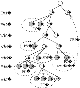
Example 2 Assume that the domains of the variables in the problem of Example 1 are as follows: D(x1) = {2, 3}, D(x2) = {0, 1, 2}, D(x3) = {0, 3}, D(x4) = {0, 1, 6}, D(x5) = {4, 5}, D(x6) = {0, 1, 2, 3}, D(x7) = {0, 2, 3, 6}. Let us trace the execution of QCSP-Solve for a few steps.

1) Preprocessing is applied. There are no arc inconsistent or pure values, so no pruning is performed. 5 2) The assignment (x1, 2) is made. FC reduces D(x6) and D(x7) to {0, 1, 3} and {0, 3, 6} respectively. We now have conf set(x6) = conf set(x7) = {x1}. 3) Now, value 2 of x2 becomes pure because it is supported by all values in future variables. The PV rule will immediately make the assignment (x2, 2). 4) FC1 does not wipe out any future domain, so the assignment (x3, 0) will be made. FC reduces D(x6) and D(x7) to {1, 3} and {3, 6} respectively. 5) Value 0 of x4 is pure. Therefore, it is removed and the assignment (x4, 1) is made. FC reduces D(x6) to {3}. 6) FC1 does not wipe out any future domain, so the assignment (x5, 4) will be made. FC reduces D(x7) to {6}. 7) x6 and x7 are assigned their only available values and a solution is found. 8) Now function SDP() is called (line 13). SDP() discovers that value 5 of the last universal (x5) is compatible with the assignments of all the existentials after x5. Therefore, this value is removed from D(x5) and a solution-directed backjump to x4 is performed. 9) The assignment (x4, 6) is made. FC reduces D(x6) and D(x7) to {1, 3} and {3} respectively. 10) FC1 applied at x5 wipes out D(x7) (value 4 of x5 is incompatible with the only value in D(x7)). Therefore, we have a dead-end. conf set(x7) will be added to conf set(x5) and the algorithm will backjump to the rightmost variable in conf set(x5), which is x1.

Figure 2 shows part of the search tree generated by QCSPSolve and illustrates how subtrees are pruned.

4 Experiments

[Gent et al., 2004] showed that the model for random generation of QCSPs used in [Mamoulis and Stergiou, 2004] can suffer from a local flaw that makes almost all of the generated instances false. In this model there are k alternating quantifiers applied to disjoint sets of variables, with the innermost quantifier being existential. Let us briefly describe the flaw. Suppose we have a series of k universals x1, . . . , xk assigned to values a1, . . . , ak respectively. If there is an existential xi later in Q than the k universals and each one of its values is in conflict with one of the values assigned to the universals then the assignment of values a1, . . . , ak to variables x1, . . . , xk is inconsistent. This assignment will remain inconsistent irrespective of the assignments to other universals or existentials, and therefore the problem is unsatisfiable. We now propose a generator that can be used to control the probability of flaws.

5 Values 4 and 5 of x5 are NI, but let us ignore this for the sake of the example.

Variables are quantified in three blocks, a block of existentials followed by a block of universals then another block of existentials.The generator takes 7 parameters: < n, n∀, npos, d, p, q∀∃, q∃∃ > where n is the total number of variables, n∀ is the number of universals, npos is the position of the first universal in Q, d is the uniform domain size, and p is the number of binary constraints as a fraction of all possible constraints. q∃∃ is the number of goods in ∃ xi∃ xj, cij constraints as a fraction of all possible tuples, and q∀∃ is a similar quantity for ∀ xi∃ xj, cij constraints, described further below. The other two types of constraints that can be removed by preprocessing are not generated.

Since the flaw is a characteristic of ∀ xi∃ xj, cij constraints, we restrict these in the following way: we generate a random total bijection from one domain to the other. All tuples not in the bijection are goods. Now q∀∃ is the fraction of goods from the d tuples in the bijection.

To control the probability pf of the flaw, we write down an expression for pf , approximating proportions p, q∀∃, q∃∃ as probabilities. n∀ is the number of universal variables, and n∃ is the number of inner existential variables. For each existential assignment (xi, a), the probability that it is covered by a universal is p(1-q∀∃). If the variable xi is flawed, then all its values are in conflict with some value of some universal variable. However, each universal variable can only cover one value (since we use a bijection). Therefore (representing existential values using integers) the probability that variable xi is flawed is given by the following.

The probability that value a is flawed, given that the previous a - 1 values are flawed, is given by formula 2.

Substituting equation (2) into equation (1) gives the probability of one variable being flawed.

The probability that no existential variables are flawed is given below. This formula is undefined when d > n∀. In this case, pf = 1.

Experimental Results

Figure 3 presents a comparison of algorithms FC1, FC1+PV, MAC1+PV, and full QCSP-Solve on problems generated according to the model described above. All algorithms apply AC, and NI preprocessing. For each value of q∃∃ shown in the figures, 100 problem instances were generated and we use the mean average. We include FC1+PV and MAC1+PV in the comparison to illustrate the power of the PV rule. In the problems of Figure 3 the execution of FC1 was stopped at the cut-off limit of 2 hours in more than 50% of the instances. As we can see, QCSP-Solve is many orders of magnitude faster than FC1. The speed-up obtained is largely due to the application of the PV rule. Similar results were obtained with various parameter settings.

Having established that QCSP-Solve is considerably faster than existing direct approaches, we compared it with the state-of-the-art approach of [Gent et al., 2004], using the adapted log encoding with the CSBJ QBF solver. Figure 4 presents indicative results of this comparison. In this case, we used the median because of high outliers. As we can see, QCSP-Solve is significantly faster than CSBJ (more than one order of magnitude), except for very high values of q∃∃.

5 Conclusion

We introduced QCSP-Solve, an efficient solver for QCSPs. QCSP-Solve incorporates a variety of techniques that are either extensions of techniques used in CSPs and QBF, or are specifically designed for QCSPs. To our knowledge, this is the first time these techniques have been devised and implemented in QCSPs. We also proposed a random generation model that can be used to create instances that are free from the flaw discovered in [Gent et al., 2004]. Experiments showed that QCSP-Solve is several orders of magnitude faster than the existing state-of-the-art direct algorithms for QCSPs, and also significantly outperforms approaches based on encoding QCSPs into QBFs. Current and future work includes extending the solver to handle constraints of any arity, and incorporating other advanced techniques, such as learning.