
A Lattice Machine Approach to Automated Casebase Design: Marrying Lazy and Eager Learning
Proceedings of the Sixteenth International Joint Conference on Artificial Intelligence. Case-based Reasoning. Pages 254-262.
© 1999 International Joint Conferences on Artificial Intelligence
Abstract
Case-based reasoning (CBR) is concerned with solving new problems by adapting solutions that worked for similar problems in the past. Years of experience in building and fielding CBR systems have shown that the "case approach" is not free from problems. It has been realized that the knowledge engineering effort required for designing many real-world casebases can be prohibitively high. Based on the wide-spread use of databases and powerful machine learning methods, some CBR researchers have been investigating the possibility of designing casebases automatica lly. This paper propo ses a flexible model for the automatic discovery of abst ract cases from databases based on the Lattice Machine. It also proposes an efficient and effective al gorithm for retrieving such cases. Besides the known benefits associated with abstract cases, the main advantages of this approac h are that the discovery process is fully automated (no knowledge engineering costs).
- [Aha, 1997] D . Aha, editor. Lazy Learning. Kluver Aca- demic Pub. , 1997.
- [Bergmann and Wilke, 1996] R. Bergmann and W . Wilke. On the role of abstraction in case- based reasoning. In Proc. Advances in Case-Based Reasoning, 3rd EWCBR-96, pages 28-41 , 1996.
- [Cohen and Hirsh, 1998] William W . Cohen and Haym Hirsh. Joins that generalize: Text classification using whirl. In Proc. KDD-98, New York, 1998.
- [Gratzer, 1978] George Gratzer. General Lattice Theory. Birkhauser, Basel, 1978.
- [Haussler, 1988] D. Haussler. Quantifying inductive bias: Ai learning algorithms and valiant's learning framework. Artifi cial Intelligence, 36:177-221, 1988.
- [Leake and Wilson, 1998] D .B. Leake and D.C. Wilson. Categorizing case base maintenance: Dimensions and directions. In Proc. Advances in Case-Based Reason- ing,4th EWCBR-98, pages 196-207, 1998.
- [Leake, 1996] D.B. Leake, editor. Case-Based Reason- ing: Experiences, Lessons fj Future Directions. MIT Press, MA, 1996.
- [Lenz et al., 1998] M. Lenz, B. Bartsch-Spi:irl, H-D. Burkhard, and S. Wess, editors. Case-Based Reas- oning Technology: From Foundations to Applications. Springer-Verlag, 1998.
- [Mitchell, 1997] T . M. Mitchell. Machine Learning. The McGraw-Hill Companies, Inc, 1997.
- [Orlowska, 1985] Ewa Orlowska. Logic of nondetermin- istic information. Studia Logica, 44:93-102, 1985.
- [Patterson et al., 1998] D. Patterson, W. Dubitzky, S.S. Anand, and J.G. Hughes. On the automation of case base development from large databases. In Proc. AAAI Workshop: Case-Based Reasoning Integrations, pages 126-130, 1998.
- [Smyth and Keane, 1995] B. Smyth and M.T. Keane. Remembering to forget: A competence-preserving case deletion policy for case-based reasoning systems. In Proc. 14th IJCAI-95, pages 337-382 , 1995. IJCAI
- [Wang et al. , 1998] Hui Wang, Ivo Diintsch, and David Bell. Data reduction based on hyper relations. In Pro- ceedings of KDD98, New York, pages 349-353, 1998.
References were extracted automatically from the PDF and may contain errors.
Full text extracted automatically from the PDF; figures, tables and equations may differ. The PDF is the version of record.
1 Introduction
Case-based reasoning (CBR) is concerned with solving new problems by adapting solutions that worked for sim ilar problems in the past. CBR research is motivated by the desire to establish cognitive models to understand human thinking and behavior (psychology, cognitive sci ence), and to build more effective, efficient, and robust computer systems that solve real-world problems (artifi cial intelligence) . Since the early nineties, CBR has been successfully applied in a wide variety of areas. However, with almost ten years of both theoretical and applied experience in building and fielding case-based systems, it has been realized that the "case approach" is not free from problems [Leake, 1996]. Two of the more important issues that need to be addressed are outlined below:
- the implementation of casebase maintenance
- policies for rev1smg the organization of casebases in order to facilitate effective and efficient future reasoning [Leake and Wilson, 1998] ; and
- the automation of the case engineering process, that is, the automatic generation of case-knowledge com ponents from existing information (i.e., databases) [Patterson et al., 1998]; the work presented in this paper will focus on this issue.
The term case engineering refers to task of designing a casebase, that is, the processes of generating those com ponents that represent the application-specific know ledge contained in a CBR system. In general, such know ledge structures describe the content structure of cases, criteria for organizing cases within and retrieving cases from the case library (indexing scheme, similarity meas ures), rules for adapting case solutions, and case revision and retention schemes [Lenz et al., 1998]. In addition to determining the fundamental knowledge elements, the generation process also entails the selection or extraction of those cases that will be used to populate the initial case base.
The work presented in this paper proposes Lattice Machine - a formal framework for learning from re lations, and its application to automatically construct (case content description) and extract (case selection) abstract cases from databases. Furthermore, an efficient algorithm for the retrieval of such abstract. cases is also proposed.
The remainder of the paper is organized as follows. Section 2 briefly discusses the role of abstract cases in CBR. Section 3 introduces the definitions and notational conventions, followed in Section 4 by a formal description of Lattice Machine, the pivotal part of the work in this paper. Sections 5 and 6 present efficient algorithms for extracting abstract cases and retrieving cases, based on the theoretical results in Lattice Machine. Experimental results are reported in Section 7. Section 8 concludes the paper.
2 Abstract Cases in CBR
Traditional CBR systems retrieve, reuse, and retain cases in a representation reflecting concrete problem solving episodes. Recently, researchers have investigated the role and use of abstract cases, e.g., [Bergmann and Wilke, 1996]. Abstract cases represent cases at a higher level of abstraction. Through abstract cases, the CBR process can be supported in several ways [Bergmann and Wilke, 1996]; those ways pertinent to the discussion in this paper are outlined below:
- Abstract cases can reduce the complexity of a case base by substituting sets of concrete cases and thereby significantly reducing the size of the case base. A drastically reduced casebase can improve retrieval efficiency, reduce maintenance costs, and eliminate or alleviate the notorious swamping prob lem [Smyth and Keane, 1995].
- Cases at higher levels of abstraction can serve as prototypes for indexing larger sets of more detailed cases. This can have profound effects on reducing retrieval times, maintenance costs, and it can pro mote a better user understanding of the casebase content, and facilitate explanations for the system's reasoning process.
In most situations, abstract cases are not readily avail able, they must be generated - manually or automatic ally - from concrete cases. To manually construct ab stract cases will require a very high knowledge engineer ing effort for most applications. Whereas an automatic generation procedure requires general domain knowledge about ways of mapping concrete cases onto higher levels of abstraction.
The abstract case construct proposed in this paper is based on the concept of hypertuples. Hypertuples, i.e., abstract cases, are automatically generated through a so-called domain lattice, which is implied in a problem domain. The extraction and retrieval of abstract cases are achieved in domain lattice using the Lattice Machine.
3 Definitions and notation
To present our findings concisely and within the given page limit, we briefly introduce some notational conven tions and definitions that are used throughout the paper.
3.1 Decision systems
An information system is a tuple I = (U, 0, Vx)xEn, where U = { a0 , ... , aN} is a nonempty finite set and f2 = { Xo, ... , XT} is a nonempty finite set of mappings X; : U --> Vx , 1 .
We interpret U as a set of objects and n as a set of attributes or features, each of which assigns to an object a its value under the respective attribute. Let V ~ f1xE!1 Vx. For a E U, we let O(a) ~ (x(a))xE!1 E V. Each O(a) is called a tuple, and the collection of all tuples is denoted by D . Thus, for each t E D, there is at least one a E U such that O(a) = t.
1 Note Vx, can be finite or infinite. For the latter case the domain lattice is infinite. However we are only interested in the finite sublattice generated from a finite casebase.
A decision system V is a pair (I, d), where I is an information system as above, and d : D _, Vd = {do, ... , dK} is an onto mapping, called a labeling of D ; the value d(t) is called the label oft.
The mapping d induces a partition Pd of D with the classes {Do, ... , DK}, where t E D ; ¢=? d(t) = d;.
In this paper we consider a dataset represented as a decision system V, which can be regarded as an initial casebase consisting of concrete cases. Then D is the set of (descriptions of) concrete cases, dis the case solution, and V is the set of all possible concrete cases in a prob lem domain. Therefore each t E D is associated with a solution in the form of a class label d(t).
3.2 Order and lattices
Let P = (P, :::;) be a partially ordered set and T ~ P. We let l T ~f {y E P : (:lx E T) y :::; x}. If no confusion can arise, we shall identify singleton sets with the element they contain.
Let L be a lattice, partially ordered by:::;. For x, y E £, the least upper bound (or sum) is written by x + y and the greatest lower bound (or product) by x x y. For A ~ L, its least upper bound and greatest lower bound are denoted by lub(A) and glb(A) respectively. An element a E A is called maximal in A, if for all x E A, a :::; x implies x = a.
For A, B ~ L, we say that B covers A or A is covered by B, written as A ~ B if for each s E A there is some t E B such that s :::; t.
The sublattice of L generated from M ~ L, written by [M], is [M] ={tEL: :JX ~ M such that t = lub(X)}. The greatest element in [M] is lub(M) . If M is finite, [M] is also finite.
A comprehensive discussion on lattice theory can be found in [Gratzer, 1978].
4 The Lattice Machine
This section introduces the Lattice Machine, a construct which facilitates the discovery of abstract cases from a given dataset. The discussion should also make apparent how the Lattice Machine is linked to machine learning concepts.
4.1 Domain lattice
We have found that, given a dataset expressed as a de cision system, an elegant mathematical structure (lat tice) is implied. This structure makes it possible to in vestigate CBR, machine learning, as well the relationship between the two from an algebraic perspective. In the sequel, we shall use V as described above as a generic decision system representing a dataset.
Let L d~f f1xE!1 2 Vx. Then t E L is a vector (t(x) )xE!1, where t(x) ~ Vx are sets of values 2 . The elements of L are called hypertuples; the elements t of L with it(x)l = 1 for all X E n are called simple tuples. Any set of hypertuples is called a hyperrelation 3 . Note that Vis a set of all simple tuples for a given problem domain, and D is the set of simple tuples described in the dataset D.
2 Note that if t E £ and x E D, then t(x) is the projection oft to its x- th component.
.C is a lattice under the ordering
with the sum and product operations, and the maximal element (i.e., 1) given by
.C is called domain lattice for D.
There is a natural embedding of D into .C by assigning
and we shall identify D with the image of this embed ding. Then D ~ V ~.C.
In the context of CBR, simple tuples are concrete cases whereas hypertuples are abstract cases since hypertuples cover multiple simple tuples hence they are "abstrac tions" of simple tuples.
Table 1 (a) is a dataset (decision system) consisting of three simple tuples, where Vx, = {a, b} and Vx 2 = {0, 1}, and dis the labeling. Table 1(b) and (c) are sets of hypertuples, which are the least and greatest E-sets respectively for the dataset, to be defined later.
II~ I
| u II x1 I x2 II d I uo a |
|---|
| 0 a |
| U1 a 1 a |
| U2 b 0 (3 |
| d |
| II~ (c) |
3 The concept of hyperrelation has been used before in e.g. [Orlowska, 1985; Wang et al., 1998].
4.2 Equilabelledness and generalization
A dataset imposes a labeling d of D on the domain lat tice .C. Thus all elements in D are labeled, and those in V \ D are unlabeled. This labeling can be gener alized to elements in the lattice which cover D . This generalization must be consistent with d in the sense that the generalized labeling must be the same as d for
t E D. This renders only those generalizations accept
able which generalize d to equilabeled elements. Intu
itively, an equilabeled element is t E .C which covers
at least one labeled element and all labeled elements
covered by t have the same label.
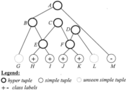
For an illustrative example, consider the diagram in Figure 1, which depicts a small part of a domain lattice. The bottom elements (thin-lined circles) in the diagram represent simple tuples. All other elements (bold-lined circles) represent hypertuples. The original labeling d is defined only for the elements {H, I , J, K , M}. Here, B is equilabeled as H and I are all labeled positive by d while G is unlabelled. In fact, all elements in Figure 1 are equilabeled except A, G and L: A covers elements with different labels whereas G and L cover no labeled element.
Formally, we call an element r E .C equilabeled with respect to Dq , if 0 #1 r n D , l r n D ~ Dq . In other words, r is equilabeled if l r intersects D , and every element in this intersection is labeled dq for some q :S K . Recall that K is the number of classes. In this case, we say that r G-belongs to Dq. We denote the set of all equilabeled elements G-belonging to Dq by Eq , and let E be the set of all equilabeled elements. Note that D ~ E, and that q, r :S K , q # r implies Eq n Er = 0.
We will now extend d over all of .C by setting
Now E, along with the extended labeling, can be re garded as a casebase of abstract cases (hypertuples). This is clearly too large. Since the elements in E are partially ordered - some are covered by some others we need only look at those which are not covered by any; they are maximal. Our wish to find maximal elements in some context leads to the following notions.
Def. 4.1. A (generalization) context (for learning) is a set P such that D S:;; P s;; V. We let
E(P) is called the E-set for P, and t E .C is said to be in context P if t E M(P).
We observe the following lemma 4 :
Lemma 4.2. A s;; B S:;; .C implies M(A) ~ M(B) and E(A) ~ E (B).
This lemma implies E (D) ~ E (P) ~ E (V ) for D S:;; P s;; V. We then call E (D ) least E-set and E (V) greatest E-set, which are denoted by E and IE respectively. It is not hard to see that IE is the set of all maximal elements in E.
Consider Figure 1 again. E( { H, · · · , K, M}) {C,M} , and E ({G,· · · ,M}) = {B,C,D,M}.
4.3 Interpretation of a domain lattice
Given a hypertuple t in a context P (i.e., t E M(P)) , we need a calculus to get the remaining hypertuples in the same context (see Theorem 4.1 below). We therefore need to interpret the domain lattice in a suitable way.
Formally, let t = (eo, ... , er) be a hypertuple, with e; = { e; 0 , ... , e;,<·J }. We think of t as an ( undetermin istic) description of some object a in the following way:
In short we have t =eo 1\ · · · 1\ ey.
Each e; stands as a hypertuple on its own, which is interpreted as (Vo, · · · , ll,;_1 , e;, Vi+l, · · · , Vr); and ejl\ek is interpreted as glb(ej, ek)·
Consider a hypertuple t = (eo , ··· , ey). The relative complement or, simply, R-complement oft with respect to the greatest element in .C (i.e., 1) is t =eo V · · · V ey, and ej is interpreted as Vj \ ej.
Given a hyperrelation R = {to,···, tn}, where t; = (e;0 , · · · , eiT), we wish to calculate its R-complement R in such a way that RuR ?= V and l Rn l R = 0. For this purpose we interpret R as to V · · · V tn. Using the propos itional calculus we can calculate the R-complement of R as follows. Let X = {1\~=0 e;j, : for j; E {0, · · · , T} }. R = 1\~=0 f; = V xEX x. If follows lXI = (T + 1)(n+l). Clearly the calculation of R-complement is exponential, which makes this not practical for large R.
The above R-complement calculus can be generalized as follows. Lett= (ew, · · · , etr) and h = (eho, · · ·, ehr). If t :S h then the R-complement of t with respect to h, denoted by tlh, is calculated similarly except that et; = ehj \ etj.
4 Due to lack of space, we omit all proofs throughout the paper.
Lemma 4.3. For R S:;; .C,
- RuR ?= V.
- l Rn l R = 0.
- Let W d~ { w E .C : l wn l R = 0}. Then R is the set of all maximal elements in W.
The first two properties guarantee that R is exclus ively complementary to R with respect to the maximal element of the domain lattice. For an example, consider Table 1(a). The table is interpreted as u0 V u 1 V u2. uo is interpreted as (X1 = a) 1\ (X2 = 0). u0 = (a, 0) = avO= (a, V2)V (V1,0). Let V1 = {a,b} and V2 = {0, 1}. Then u0 = (b,{0,1})v ({a,b},1), which clearly covers u 1 and u2, as well as an unseen tuple (b, 1).
The third property says that R is the set of maximal elements not covered by R. Consider Figure 1. Let R = {E}. Then R = {G, D, M}.
4.4 Hypothesis space and casebase
Given a dataset we wish to have a hypothesis to replace the entire dataset. The hypothesis should not only cover the dataset but also generalize it. As discussed earlier, a dataset V imposes a labeling on the underlying domain lattice. The labeling can then be generalized to elements in M(P) for a given context P. However we do not need to use the whole M(P) as the hypothesis; a proper subset of it will suffice. Then a hypothesis is just a set of hypertuples, each of which is more informative than the simple tuples in the original dataset. Therefore, it is possible to consider a casebase as a hypothesis for a dataset. In this section we will introduce and justify some concepts through which we can precisely describe what kind of hypothesis we are aiming for.
Note that, by Lemma 4.2, M(D) ~ M(P) ~ M(V) for D S:;; P S:;; V. Therefore H s;; M(P) => H s;; M(V). Then we have
Def. 4.4. A hypothesis for D is a H S:;; M(V) such that D ~ H . We use GEN(D) to denote the set of all hypo theses for V.
Similarly, we define a hypothesis for Dq· Note that for a hypothesis H for D, H n Eq is a hypothesis for Dq. Conversely, if Hq is a hypothesis for Dq for each q :S K , then H ~ U <K Hq is a hypothesis for D. q_
Since M(P) contains only equilabeled elements, His consistent with the dataset. Since D ~ H, H covers all simple tuples in the dat?Set.
Def. 4.5. Let Hi and Hk be two hypotheses for D. Then Hi is more general than H k if and only if H k ~ Hi. Hj is (strictly) more general than Hk, written (Hk-< HJ) , if and only if (Hk ~ HJ) 1\ (HJ 1;. Hk)·
A hypothesis H for D is maximally general if and only if H E GEN(D) and there is no H' E GEN(D) such that H -< H'. We denote by G the set of all maximally general hypotheses for D . In [Mitchell, 1997] G is called the general boundary for D.
The following lemma establishes the equivalence between G and the greatest E-set (IE).
Lemma 4.6. G = {lE}.
This lemma says that, although there are many pos sible hypotheses for a given dataset, there is only one maximally general hypothesis - the greatest E-set. This hypothesis is consistent with the dataset but has the maximal coverage of unseen simple tuples (because it has the maximal context V). General boundary is a well established concept in the field of concept learn ing, and it has been used as an inductive bias in some concept learning algorithms [Mitchell, 1997]. The equi valence of the greatest E-set and the general boundary enables us to use the same inductive bias in automatic casebase design. Therefore our objective is to find the greatest E-set for a dataset. Our casebase design and retrieval are both associated with the greatest E-set.
However, as shown in [Haussler, 1988], the size of the general boundary can grow exponentially in the number of training examples. In the context of domain lattice, calculating the greatest E-set needs V, which is not ex plicitly available; instead it has to be calculated from D using the R-complement calculus discussed above. This involves calculating D , which has been shown exponen tial in ID I· It is then not practical to directly use the greatest E-set as the casebase. The following theorem guarantees that we can use a much smaller hypothesis as the casebase, but we can still use the general boundary as inductive bias. In effect it establishes the relationship between the casebase and the greatest E-set.
Theorem 4.1. Let H be hypothesis for 'D, as defined in Def. 4.4. Let VIE =1 lE n V, and VH {t E V : :lh E H,:lg E (hlh+t) U h, such that t :::; g, and g is equilabeled or unknown} . Then VIE S::: V H.
This theorem says that if a case (simple tuple) t is covered by lE, then there must be h such that t :::; h or t :::; g for g E hih + t with g being either equilabeled or unknown. Note that hih + t is the R-complement of h with respect to h + t , which is the set of all elements covered by h + t but not covered by h. The CASERE TRIEVE algorithm in Section 6 exploits this theorem to retrieve cases to classify new cases.
Theorem 4.1 says that any hypothesis can be used as a casebase that serves as an intermediary between a new case and the greatest E-set. Classification of a new case can then be made based on its relationship to the greatest E-set , which employs the general boundary inductive bias.
5 Case extraction
As indicated in Theorem 4.1, an expected case base can be any hypothesis as defined in Def. 4.4. The simplest one is the dataset itself. However, checking whether the conditions are satisfied requires computing R-complements of the tuples. It is usually the case that datasets are large hence the computation cost is high. Therefore we need an algorithm to efficiently find a hy pothesis, other than the dataset itself, satisfying the conditions. The least E-set seems ideal since it is the E-set in the minimal context (D). However calculating the least E-set is computationally expensive. The following algorithm, CASEEXTRACT, finds, given the minimal con text D, the set of elements in M(D) which have disjoint coverage of D.
Given Dq and Eq as defined above.
- Initialization: let X= Dq, H = 0.
- Repeat until X is empty:
- Let h E X and X = X \ { h}.
- ForgE X, let X= X \ g. If h+g is equilabeled then h = h +g.
- Let H = H u { h}.
This algorithm bi-partitions X into a set of elements the sum of which is an equilabeled element, and a new X consisting of the rest of the elements. The new X is similarly hi-partitioned until X becomes empty. This process leads to a binary tree, the depth of which is a measure of the time complexity of the algorithm. In the worst case the time complexity for building the casebase for class Dq is in the order of O(IDql). Therefore the worst case complexity for building the whole casebase is O(K x IDql), where K is the number of classes.
Consider Figure 1. CASEEXTRACT gives the hy pothesis { E, F, M} which has disjoint coverage of the labeled elements.
6 Case retrieval
The retrieval of relevant cases from the case base is argu ably the most important process in CBR. In this section we discuss how to retrieve cases from a casebase to clas sify new instances. Having a casebase H as discovered by the CASEEXTRACT algorithm, we can associate a new instance t E V with a case hE H by checking whether t is covered by lE through h. Then t is regarded as being in the same class as h. The CASERETRIEVE algorithm is as follows.
- Sort the elements in H in decreasing order of lXI for h E H and h = lub(X), which results in H = {ho, · · · , hn} with ho having the largest coverage of D elements.
- t is classified by the first hi in the sorted H such that the conditions in Theorem 4.1 are satisfied.
- If there is no such hi, label t by d(h0 ).
The time complexity of this algorithm is dominated by calculating the R-complement of h E H, as needed in Theorem 4.1. This is in the order of O(T), where T is the number of attributes. In the worst case we need to do so for all hi in H, i = 0, · · · , n. Therefore the overall time complexity of the algorithm is O(nT) in the worst case.
To illustrate the CASERETRIEVE algorithm, consider Figure 1. The casebase is now {E, F, M}, as discovered by CASEEXTRACT. Consider a new case G. The sum of G and E is B , which is equilabeled. Then E is retrieved and G is labeled as positive. Clearly G < B , hence �~lE.
7 Experiment
CASEEXTRACT and CASERETRIEVE are implemented in our CBR system, called LM. We compared LM with C4.5 using public datasets. The datasets are described in Table 2. Datasets in the upper half are from UC Irvine Machine Learning Repository; and those in the lower half are collections of documents which are used as benchmark for text mining study [Cohen and Hirsh, 1998]. The results are shown in Table 3.
| Datasets | #Features #Terms | #Train | # Test | #Class |
|---|---|---|---|---|
| Annealing Auto Diabetes Glass Iris Sonar Vote Memos CD roms Birdcom Birdsci | 38 25 8 9 4 60 18 1014 1133 674 1738 | 798 205 768 214 150 208 232 334 798 914 914 | 5cv 5cv 5cv 5cv 5cv 5cv 5cv lOcv lOcv lOcv 10cv | 6 6 2 6 3 2 2 11 6 22 22 |
| Dataset | Prediction accuracy | |
|---|---|---|
| C4.5 | LM | |
| Annealing | 91.8 | 93.6 |
| Auto | 72.2 | 76.1 |
| Diabetes | 72.9 | 71.7 |
| Glass | 81.3 | 82.7 |
| Iris | 94.0 | 96.0 |
| Sonar | 69.4 | 69.7 |
| Vote | 95. 1 | 97.0 |
| memos cdr oms | 57.5 | 59.8 40.0 |
| 39.2 | ||
| bird com | 79.6 | 90.4 |
| birdsci | 83.3 | 92.3 |
| Average | 76.0 | 79.0 |
8 Summary and conclusion
The paper proposed a promising model for automating the design of CBR systems. Revolving around the no tion of hypertuples (abstract cases), the proposed model presents a successful attempt at combining powerful eager techniques from machine learning with the flex ible "defer-processing" philosophy characteristic for lazy methods [Aha, 1997]. On the basis of concise formal argument and empirical evaluation, it has been demon strated that the Lattice Machine approach constitutes an effective and efficient mechanism to discover abstract cases in a given dataset. Abstract cases have been shown to be an effective alternative to representing the know ledge held in CBR systems [Bergmann and Wilke, 1996] .
They can provide answers to issues such as casebase complexity, maintenance costs, retrieval efficiency, and user acceptance. In addition to the discovery of abstract cases, an algorithm was presented, which employs the general boundary inductive bias and ensures that the retrieval of relevant abstract cases is within the limits of reasonable time constraints. The main contribution of this work lies in the Lattice Machine's ability to discover abstract cases within a given dataset without requiring difficult-to-obtain domain knowledge.
@inproceedings{ijcai1999p38,
  title     = {A Lattice Machine Approach to Automated Casebase Design: Marrying Lazy and Eager Learning},
  author    = {Wang, Hui and Dubitzky, Werner and Düntsch, Ivo and Bell, David A.},
  booktitle = {Proceedings of the Sixteenth International Joint Conference on
               Artificial Intelligence, {IJCAI-99}},
  publisher = {International Joint Conferences on Artificial Intelligence},
  editor    = {Thomas Dean},
  pages     = {254--262},
  year      = {1999},
  note      = {Case-based Reasoning},
  url       = {https://ijcai.org/proceedings/1999/38},
}
TY - CPAPER TI - A Lattice Machine Approach to Automated Casebase Design: Marrying Lazy and Eager Learning AU - Wang, Hui AU - Dubitzky, Werner AU - Düntsch, Ivo AU - Bell, David A. T2 - Proceedings of the Sixteenth International Joint Conference on Artificial Intelligence, IJCAI-99 PB - International Joint Conferences on Artificial Intelligence PY - 1999 SP - 254 EP - 262 UR - https://ijcai.org/proceedings/1999/38 ER -Copied
Machine-readable versions of this paper, for tools and AI agents:





