
AND/OR Cutset Conditioning
Proceedings of the Nineteenth International Joint Conference on Artificial Intelligence. Pages 230-234.
© 2005 International Joint Conferences on Artificial Intelligence
Abstract
Cutset conditioning is one of the methods of solving reasoning tasks for graphical models, especially when space restrictions make inference (e.g., jointree-clustering) algorithms infeasible. The wcutset is a natural extension of the method to a hybrid algorithm that performs search on the conditioning variables and inference on the remaining problems of induced width bounded by w. This paper takes a fresh look at these methods through the spectrum of AND/OR search spaces for graphical models. The resulting AND/OR cutset method is a strict improvement over the traditional one, often by exponential amounts.
- [Bayardo and Miranker, 1996] R. Bayardo and D. Miranker. A complexity analysis of space-bound learning algorithms for the constraint satisfaction problem. In AAAI'96, 1996.
- [Bidyuk and Dechter, 2003] B. Bidyuk and R. Dechter. Cycle-cutset sampling for bayesian networks. In The Canadian AI Conference, (CAAI'03), 2003.
- [Bidyuk and Dechter, 2004] B. Bidyuk and R. Dechter. On finding minimal w-cutset problem. In UAI'04, 2004.
- [Darwiche, 2001] A. Darwiche. Recursive conditioning. Ar- tificial Intelligence Journal, 125(1-2):5-41, 2001.
- [Dechter and Mateescu, 2004] R. Dechter and R. Mateescu. Mixtures of deterministic-probabilistic networks and their AND/OR search space. In UAI'04, 2004.
- [Dechter, 1990] R. Dechter. Enhancement schemes for con- straint processing: Backjumping, learning and cutset de- composition. Artificial Intelligence, 41:273-312, 1990.
- [Dechter, 1999] R. Dechter. Bucket elimination: A unifying framework for reasoning. Artificial Intelligence, pages 41- 85, 1999.
- [Fishelson and Geiger, 2002] M. Fishelson and D. Geiger. Exact genetic linkage computations for general pedigrees. Bioinformatics, 18(1):189-198, 2002.
- [Freuder and Quinn, 1985] E. C. Freuder and M. J. Quinn. Taking advantage of stable sets of variables in constraint satisfaction problems. In IJCAI'85, 1985. IJCAI
- [Kjæaerulff, 1990] U. Kjæaerulff. Triangulation of graph- based algorithms giving small total state space. Technical report, University of Aalborg, Denmark, 1990.
- [Larrosa and Dechter, 2002] J. Larrosa and R. Dechter. Boosting search with variable-elimination. Constraints, pages 407-419, 2002.
- [Pearl, 1988] J. Pearl. Probabilistic Reasoning in Intelligent Systems. Morgan Kaufmann, 1988.
- [Rish and Dechter, 2000] I. Rish and R. Dechter. Resolution vs. search; two strategies for sat. Journal of Automated Reasoning, 24(1/2):225-275, 2000.
References were extracted automatically from the PDF and may contain errors.
Full text extracted automatically from the PDF; figures, tables and equations may differ. The PDF is the version of record.
1 Introduction
Graphical models are a widely used knowledge representation framework that captures independencies in the data and allows for a concise representation. The complexity of a reasoning task over a graphical model depends on the induced width of the graph. For inference-type algorithms, the space complexity is exponential in the induced width in the worst case, which often makes them infeasible for large and densely connected problems. In such cases, space can be traded at the expense of time by conditioning (assigning values to variables). Search algorithms perform conditioning on all the variables. Cycle-cutset schemes [Pearl, 1988; Dechter, 1990] only condition on a subset of variables such that the remaining network is singly connected and can be solved by inference tree algorithms. The more recent hybrid w-cutset scheme [Rish and Dechter, 2000; Bidyuk and Dechter, 2003] conditions on a subset of variables such that, when removed, the remaining network has induced width w or less, and can be solved by a variable elimination [Dechter, 1999] type algorithm.
The AND/OR search space for graphical models [Dechter and Mateescu, 2004] is a newly introduced framework for search that is sensitive to the independencies in the model, often resulting in exponentially reduced complexities. The traditional way of doing search consists of instantiating the n variables of the problem as if they were all connected in a chain, which results in a search tree exponential in n. In contrast, AND/OR search is based on a pseudo tree which expresses independencies between variables, resulting in a search tree exponential in the depth m of the pseudo tree, where clearly m ≤ n.
This paper applies the AND/OR paradigm to the cycle cutset method. We show that the AND/OR cycle cutset is a strict improvement of the traditional cycle cutset method (and the same holds for the extended w-cutset version). The result goes beyond the simple organization of the traditional cutset in an AND/OR pseudo tree, which would be just the straightforward improvement. The complexity of exploring the traditional cutset is time exponential in the number of nodes in the cutset, and therefore it calls for finding a minimal cardinality cutset C. The complexity of exploring the AND/OR cutset is time exponential in its depth, and therefore it calls for finding a minimal depth AND/OR cutset AO-C. That is, a set of nodes that can be organized in a start pseudo tree of minimal depth. So, while the cardinality of the optimal AND/OR cutset, |AO-C|, may be far larger than that of the optimal traditional cutset, |C|, the depth of AO-C is always smaller than or equal to |C|.
2 Preliminaries
Reasoning graphical models A reasoning graphical model is a triplet R = (X,D, F) where X is a set of variables, X = {X1, . . . ,Xn}, D = {D1, . . . ,Dn} is the set of their respective finite domains and F = {F1, . . . , Ft} is a set of real-valued functions, defined over subsets of X. The primal graph of a reasoning problem has a node for each variable, and any two variables appearing in the same function's scope are connected. The scope of a function is its set of arguments. Belief networks A belief network can be viewed as an instance of a reasoning graphical model. In this case the set of functions F is denoted by P = {P1, . . . , Pn} and represents a set of conditional probability tables (CPTs): Pi = P(Xi|pai), where pai are the parents of Xi. The associated directed graph G, drawn by pointing arrows from parents to children, should be acyclic. The belief network represents a probability distribution over X having the product form PB(¯x) = P(x1, . . . , xn) = Π n i=1 P(xi|xpai ). The moral graph of a directed graph is the undirected graph obtained by connecting the parent nodes of each variable and eliminating direction.
Constraint networks A constraint network can also be viewed as an instance of a reasoning graphical model. In this case the functions are denoted by C = {C1, ..., Ct}, and the constraint network is denoted by R = (X, D, C). Each constraint is a pair Ci = (Si,Ri), where Si ⊆ X is the scope of the relation Ri that denotes the allowed combinations of values.
Induced-graphs and induced width An ordered graph is a pair (G, d), where G is an undirected graph, and d = X1, ...,Xn is an ordering of the nodes. The width of a node in an ordered graph is the number of the node's neighbors that precede it in the ordering. The width of an ordering d, denoted w(d), is the maximum width over all nodes. The induced width of an ordered graph, w ∗ (d), is the width of the induced ordered graph obtained as follows: nodes are processed from last to first; when node X is processed, all its preceding neighbors are connected. The induced width of a graph, w ∗ , is the minimal induced width over all its orderings. The tree-width of a graph is the minimal induced width. The path-width pw ∗ of a graph is the tree-width over the restricted class of orderings that correspond to chain decompositions.
3 AND/OR Search Spaces for Graphical Models
This section introduces the basics of AND/OR search spaces for graphical models as presented in [Dechter and Mateescu, 2004]. Given a graphical model R = (X,D, F), its AND/OR search space is driven by a pseudo tree [Freuder and Quinn, 1985]:
DEFINITION 1 (pseudo tree) Given an undirected graph G = (V,E), a directed rooted tree T = (V,E ′ ) defined on all its nodes is called pseudo tree if any arc of G which is not included in E ′ is a back-arc, namely it connects a node to an ancestor in T .
3.1 AND/OR Search Tree
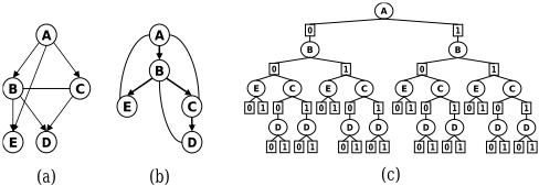
Given a graphical model R = (X,D, F), its primal graph G and a pseudo tree T of G, the associated AND/OR search tree, denoted ST (R), has alternating levels of AND and OR nodes. The OR nodes are labeled Xi and correspond to the variables. The AND nodes are labeled 〈Xi, xi〉 and correspond to the value assignments in the domains of the variables. The structure of the AND/OR search tree is based on the underlying backbone tree T. The root of the AND/OR search tree is an OR node labeled with the root of T .
The children of an OR node Xi are AND nodes labeled with assignments 〈Xi, xi〉 that are consistent with the assignments along the path from the root, path(xi) =
(〈X1, x1〉, 〈X2, x2〉, . . . , 〈Xi-1, xi-1〉). Consistency is well defined for constraint networks. For probabilistic networks, consistent tuples have non zero probability.
The children of an AND node 〈Xi, xi〉 are OR nodes labeled with the children of variable Xi in the pseudo tree T .
Example 1 Figure 1a shows a belief network. Figure 1b shows a pseudo tree of the moral graph, together with the back-arcs (dotted lines). Figure 1c shows the AND/OR search tree based on the pseudo tree, for binary valued variables.
The AND/OR Search Tree can be traversed by a depth first search algorithm. The arcs from Xi to 〈Xi, xi〉 are associated with appropriate labels of the functions in F. The algorithmmaintains values for each node, accumulating the result of the computation performed in the subtree below. The computation is dictated by the graphical model and task at hand, for example for belief networks, AND nodes are associated with multiplication (of the values of the independent subproblems) and OR nodes are associated with summation (over all the values of the variable). Based on earlier work [Freuder and Quinn, 1985; Bayardo and Miranker, 1996; Darwiche, 2001], it can be shown that:
THEOREM 1 Given a graphical model R and a pseudo tree T of depth m, the size of the AND/OR search tree based on T is O(n · exp(m)). A graphical model of tree-width w ∗ has an AND/OR search tree of size O(exp(w ∗ · log n)).
3.2 AND/OR Search Graph
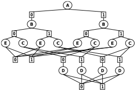
The AND/OR search tree may contain nodes that root identical subtrees. These are called unifiable. When unifiable nodes are merged, the search space becomes a graph. Its size becomes smaller at the expense of using additional memory. In this way, the depth first search algorithm can be modified to cache previously computed results, and retrieve them when the same nodes are encountered again. Some unifiable nodes can be identified based on their contexts [Darwiche, 2001]. The context of an AND node 〈Xi, xi〉 is defined as the set of ancestors of Xi in the pseudo tree, including Xi, that are connected to descendants of Xi. It is easy to verify that the context of Xi d-separates [Pearl, 1988] the subproblem below Xi from the rest of the network. The context minimal AND/OR graph is obtained by merging all the context unifiable AND nodes.
Example 2 Figure 2 shows the context-minimal AND/OR search graph of the problem and pseudo tree from Figure 1.
It can be shown that [Bayardo and Miranker, 1996; Dechter and Mateescu, 2004]:
THEOREM 2 Given a graphical model R, its primal graph G and a pseudo tree T , the size of the context minimal AND/OR search graph based on T is O(exp(w ∗ T (G))), where w ∗ T (G) is the induced width of G (extended with the pseudo tree extra arcs) over the ordering given by the depth first traversal of T .
4 Cycle Cutset Explored by AND/OR Search
The AND/OR paradigm exploits the problem structure, by solving independent components separately. This fundamental idea can also be applied to the cycle cutset method, or reasoning by conditioning [Pearl, 1988].
DEFINITION 2 (cycle cutset) Given a graphical model R = (X, D, F ), a cycle cutset is a subset C ⊂ X such that the primal graph of R becomes singly connected if all the nodes in C are removed from it. An optimal cycle cutset is one having the minimum number of variables.
The cycle cutset method consists of enumerating all the possible instantiations of C, and for each one of them solving the remaining singly connected network by a linear time and space tree algorithm. The instantiations of C are enumerated by regular OR search, yielding linear space complexity and O(exp |C|) time complexity, therefore requiring a minimal cycle cutset to optimize complexity.
A first simple improvement to the traditional cycle cutset scheme described above would be the enumeration of C by AND/OR search.
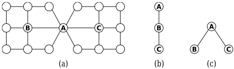
Example 3 Figure 3a shows two 3 × 3 grids, connected on the side node A. A cycle cutset must include at least two nodes from each grid, so the minimal cycle cutset contains three nodes: the common node A and one more node from each grid, for example B and C. The traditional way of solving the cycle cutset problem consists of enumerating all the assignments of the cycle cutset {A,B,C}, as if these variables form the chain pseudo tree in Figure 3b. However, if A is the first conditioning variable, the remaining subproblem is split into two independent portions, so the cycle cutset {A, B, C} can be organized as an AND/OR search space based on the pseudo tree in Figure 3c. If k is the maximum domain size of variables, the complexity of solving Figure 3b is O(k 3 ) while that of solving Figure 3c is O(k 2 ).
We can improve the general cycle cutset method, based on the previous example: first find the minimal cycle cutset C; then find the minimal depth start pseudo tree made of nodes in C:
DEFINITION 3 (start pseudo tree) Given an undirected graph G = (V,E), a directed rooted tree T = (V ′ ,E ′ ), where V ′ ⊆ X, is called a start pseudo tree if it has the same root and is a subgraph of some pseudo tree of G.
If a cycle cutset of cardinality |C| = c is explored by AND/OR search, based on a start pseudo tree T over the set C, and the depth of T is m, then m ≤ c. Therefore,
Proposition 1 Exploring a cycle cutset by AND/OR search is always better than, or the same as, exploring it by OR search.
5 AND/ORCycle Cutset
The idea presented in section 4 is a straightforward application of the AND/OR paradigm to cycle cutsets. In the following we will describe a more powerful version of the AND/OR cycle cutset.
DEFINITION 4 (AND/OR cycle cutset) Given a graphical model R = (X,D, F), an AND/OR cycle cutset AO-C is a cycle cutset together with an associated start pseudo tree TAO-C of depth m. An optimal AND/OR cycle cutset is one having the minimum depth m.
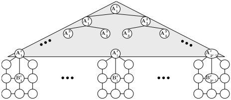
Example 4 Figure 4 shows a network for which the optimal cycle cutset contains fewer nodes than the optimal AND/OR cycle cutset, yet the latter yields an exponential improvement in time complexity. The network in the example is based on a complete binary tree of depth r, the nodes marked A j i shown on a gray background. The upper index j corresponds to the depth of the node in the binary tree, and the lower index i to the position in the level. Each of the leaf nodes, from A r 1 to A r 2 r-1 is a side node in a 3 × 3 grid. A cycle cutset has to contain at least 2 nodes from each of the 2 r-1 grids. An optimal cycle cutset is C = {A r 1 , . . . ,A r 2 r-1 , B r 1 , . . . ,B r 2 r-1}, containing 2 r nodes, so the complexity is O(exp |C|) = O(exp(2 r )). We should note that the best organization of C as an AND/OR space would yield a pseudo tree of depth 2 r-1 +1. This is because all the nodes in {A r 1 , . . . ,A r 2 r-1} are connected by the binary tree, so they all must appear along the same path in the pseudo tree (this observation also holds for any other optimal cycle cutset in this example). Exploring C by AND/OR search lowers the complexity from O(exp(2 r )) to O(exp(2 r-1 +1)).
Let's now look at the AND/OR cycle cutset AO-C = {A j i | j = 1, . . . , r; i = 1, . . . , 2 j-1 } ∪ {B r 1 , . . . ,B r 2 r-1}, containing all the A and B nodes. A pseudo tree in this case is formed by the binary tree of A nodes, and the B nodes exactly in the same position as in the figure. The depth in this case is r + 1, so the complexity is O(exp(r + 1)), even though the number of nodes is |AO-C| = |C| + 2 r-1 - 1.
The previous example highlights the conceptual difference between the cycle cutset method and what we will call the AND/OR cycle cutset method. In cycle cutset, the objective is to identify the smallest cardinality cutset. Subsequently, the exploration can be improved from OR search to AND/OR search. In AND/OR cycle cutset the objective is to find a cutset that forms a start pseudo tree of smallest depth.
THEOREM 3 Given a graphical model R, an optimal cycle cutset C, its corresponding smallest depth start pseudo tree TC , and the optimal AND/OR cycle cutset AO-C with the start pseudo tree TAO-C, then:
There exist instances for which the inequalities are strict.
We should note that strict inequalities in Eq. 1 could translate into exponential differences in time complexities.
6 AND/OR w-Cutset
The principle of cutset conditioning can be generalized using the notion of w-cutset. A w-cutset of a graph is a set of nodes such that, when removed, the remaining graph has induced width at most w. A hybrid algorithmic scheme combining conditioning and w-bounded inference was presented in [Rish and Dechter, 2000; Larrosa and Dechter, 2002]. More recently, w-cutset sampling was investigated in [Bidyuk and Dechter, 2003], and the complexity of finding the minimal w-cutset was discussed in [Bidyuk and Dechter, 2004].
The hybrid w-cutset algorithm performs search on the cutset variables and exact inference (e.g. bucket elimination [Dechter, 1999]) on each of the conditioned subproblems. If the w-cutset Cw is explored by linear space OR search, the time complexity is O(exp(|Cw| + w)), and the space complexity is O(expw).
The AND/OR cycle cutset idea can be extended naturally to AND/OR w-cutset. To show an example of the difference between the traditional w-cutset and the AND/OR w-cutset we refer again to the example in Figure 4. Consider each 3 × 3 grid replaced by a network which has a minimal wcutset Cw. The minimal w-cutset of the whole graph contains in this case 2 r-1 · |Cw| nodes. If this w-cutset is explored by OR search, it yields a time complexity exponential in (2 r-1 · |Cw| +w). If the w-cutset is explored by AND/OR search it yields a time complexity exponential in (2 r-1 + |Cw| + w) (similar to Example 4). In contrast to this, the AND/OR wcutset, which contains the A nodes and the w-cutsets of each leaf network, yields a time complexity exponential only in (r + |Cw| +w), or possibly even less if the nodes in Cw can be organized in a start pseudo tree which is not a chain (i.e. has depth smaller than |Cw|).
7 AlgorithmDescription
The idea of w-cutset schemes is to define an algorithm that can run in space O(expw). The AND/OR w-cutset algorithm is a hybrid scheme. The cutset portion, which is organized in a start pseudo tree, is explored by AND/OR search. The remaining w-bounded subproblems can be solved either by a variable elimination type algorithm, or by search with wbounded caching - in particular, AND/OR search with full caching is feasible for these subproblems.
7.1 Improved AND/ORCaching Scheme
In [Dechter and Mateescu, 2004], the caching scheme of AND/OR search is based on contexts [Darwiche, 2001], which are precomputed based on the pseudo tree before search begins. Algorithm AO(i) performs caching only at the variables for which the context size is smaller than or equal to i (called i-bound).
The cutset principle inspires a more refined caching scheme for AO, which caches some values even at nodes with contexts greater than the i-bound. Lets assume the context of the node Xk is context(Xk) = {X1, . . . , Xk}, where k > i. During the search, when variables X1, . . . ,Xk-i are instantiated, they can be regarded as part of a cutset. The problem rooted by Xk-i+1 can be solved in isolation, like a subproblem in the cutset scheme, after the variables X1, . . . ,Xk-i are assigned their current values in all the functions. In this subproblem, context(Xk) = {Xk-i+1, . . . ,Xk}, so it can be cached within i-bounded space. However, when the search retracts to Xk-i or above, the cache table for variable Xk needs to be purged, and will be used again when a new subproblem rooted at Xk-i+1 is solved.
This improved caching scheme only increases the space requirements linearly, compared to AO(i), but the time savings can be exponential. We will show results in section 8.
7.2 AlgorithmAO-C(i)
We can now define the different versions of AND/OR i-cutset algorithm that we experimented with. We chose to explore the cutset portion either by linear space AND/OR search (no caching) or by AND/OR search with improved caching. For the i-bounded subproblems, we chose either Bucket Elimination (BE) or AND/OR search with full caching (which coincides with the improved caching on the bounded subproblems). The four resulting algorithms are: 1) AO-LC(i) - linear space cutset and full caching for subproblems; 2) AO-LC-BE(i) - linear space cutset and BE for subproblems; AO-C(i) - improved caching everywhere; 4) AO-C-BE(i) - improved caching on cutset and BE on subproblems.
7.3 Finding a Start Pseudo Tree
The performance of AO-C(i) is influenced by the quality of the start pseudo tree. Finding the minimal depth start pseudo tree for the given i-bound is a hard problem, and it is beyond the scope of this paper to address its complexity and solution. We will only describe the heuristic we used in creating the pseudo trees for our experiments.
Min-Fill [Kjæaerulff, 1990] is one of the best and most widely used heuristics for creating small induced width orderings. The ordering defines a unique pseudo tree. The minimal start pseudo for an i-bound contains the nodes for which some descendant has adjusted context (i.e. context without the variables instantiated on the current path) greater than i. Min-Fill heuristic tends to minimize context size, rather than pseudo tree depth. Nevertheless, we chose to try it and discovered that it provides one of the best pseudo trees for higher values of i.
| CPCS 422 - f(i) | |||||||||||
|---|---|---|---|---|---|---|---|---|---|---|---|
| i | 1 | 2 | 3 | 4 | 5 | 6 | 7 | 8 | 9 | 10 | 11 |
| d(AO-C) | 32 | 32 | 32 | 32 | 31 | 31 | 31 | 31 | 31 | 30 | 29 |
| d(C) | 40 | 37 | 32 | 32 | 38 | 37 | 36 | 34 | 32 | 30 | 29 |
| |C| | 79 | 71 | 65 | 59 | 54 | 50 | 46 | 41 | 37 | 34 | 32 |
| GWCA | 79 | 67 | 60 | 55 | 50 | 46 | 42 | 38 | 34 | 31 | 29 |
Min-Depth We developed a heuristic to produce a balanced start pseudo tree, resulting in smaller depth. We start from a Min-Fill tree decomposition and then iteratively search for the separator that would break the tree in parts that are as balanced as possible, relative to the following measure: on either side of the separator eliminate the separator variables, count the number of remaining clusters, say n, and then add the sizes of the largest logn clusters.
GWC [Bidyuk and Dechter, 2004] is a greedy algorithm to build a minimal cardinality cutset. In the process, we also arranged the minimal cardinality cutset as AND/OR cutset, to compare with the minimal depth cutset that we could find.
8 Experimental Evaluation
We investigated two directions. One was to empirically test the quality of the start pseudo trees, and the other was to compare actual runs of the different versions of AO-C(i).
8.1 The Quality of Start Pseudo Trees
We report here the results on the CPCS 422b network from the UAI repository. It has 422 nodes and induced width 22. Table 1 shows the values of f(i), which expresses the total complexity of a cutset scheme. For a cardinality cutset, f(i) = i + |C| and for an AND/OR cutset of depth d, f(i) = i + d. The row d(AO-C) shows the depth of the best AND/OR cutset we could find. |C| shows the number of nodes in the best cutset found by GWC, and d(C) shows its depth when organized as AND/OR cutset. GWCA is taken from [Bidyuk and Dechter, 2004]. The best complexity, expressed by small values of f(i), is always given by the AND/OR cutset, and for smaller values of i they translate into impressive savings over the cardinality cutset C.
In all our experiments described in the following, we refrained from comparing the new cutset scheme with the old cardinality cutset scheme (equivalent to an OR search on the cutset), because the latter was too slow.
8.2 Performance of AO-C(i)
We tested the different version of the AO-C(i) family primarily on Bayesian networks with strictly positive distributions, for the task of belief updating. This is necessary to grasp the power of the scheme when no pruning is involved in search.
In all the tables N is the number of nodes, K is the maximum domain size, P is the number of parents of a variable, w ∗ is the induced width, i is the i-bound, d is the depth of the i-cutset. For most problems, we tested a min-fill pseudo-tree (MF) and one based on the depth minimizing heuristic (MD).
| N=40, K=3, P=2, 20 instances, w*=7 | |||||||
|---|---|---|---|---|---|---|---|
| i | Algorithms | d | Time(sec) | # nodes | |||
| MF | MD | MF | MD | MD | MF | ||
| 1 | AO(i) AO-LC(i) AO-C(i) AO-C-BE(i) | 12 | 9 | 610.14 174.53 67.99 16.95 | 27.12 8.75 7.61 2.18 | 50,171,141 13,335,595 4,789,569 - | 1,950,539 575,936 499,391 - |
| 3 | AO(i) AO-LC(i) AO-C(i) | 7 | 6 | 71.68 5.73 2.94 0.69 | 8.13 0.84 0.84 0.25 | 5,707,323 501,793 248,652 - | 595,484 69,357 69,357 - |
| 5 | AO-C-BE(i) AO(i) AO-LC(i) AO-C(i) AO-C-BE(i) | 4 | 3 | 11.28 0.55 0.55 0.10 | 2.77 0.54 0.55 0.04 | 999,441 50,024 49,991 - | 24,396 4,670 4,670 - |
| N=60, K=3, P=2, 20 instances, w*=11 | |||||||
| i | Algorithms | d | Time(sec) | # nodes | |||
| MD | |||||||
| MF | MD | MF | MD | MF | |||
| 6 | AO-LC(i) AO-C(i) AO-C-BE(i) | 7 | 6 | 159.79 112.43 | 63.01 62.98 | 14,076,416 9,925,855 - | 5,165,486 5,165,486 |
| 9 | AO-LC(i) AO-C(i) | 3 | 27.33 24.40 | 5.50 41.45 | - 3,509,709 | ||
| AO-C-BE(i) | 3 | 24.15 4.27 17.39 | 40.93 2.89 38.46 | 2,140,791 2,140,791 - | 3,509,709 - | ||
| 11 | AO-LC(i) AO-C(i) | 0 | 1 | 17.66 | 38.22 | 1,562,111 1,562,111 | 3,173,129 3,173,129 |
| AO-C-BE(i) | 1.29 | 2.81 | - | - | |||
The time and the number of nodes expanded in the search are shown for the two pseudo trees correspondingly.
Random networks. Table 2 shows results for random networks, generated based on N, K and P and averaged over 20 instances. Note that K=3, which makes the problems harder, even though w ∗ seems small. For N=40 we see that the old scheme AO(i) is always outperformed. Using improved caching on the cutset is almost always beneficial. For i very close to w∗, caching on the cutset doesn't save much, and in some cases when no caching is possible, the extra overhead may actually make it slightly slower. Also, for strictly positive distributions, switching to BE is faster than running AO search with caching on the remaining problems.
CPCS networks. CPCS are real life networks for medical diagnoses, which are hard for belief updating. Table 3 shows results for CPCS 360 file, having induced width 20. For i = 20, AO-C-BE(i) is actually BE. It is interesting to note that AO-LC-BE(i), for i = 12 is actually faster than BE on the whole problem, while requiring much less space (exp(12) compared to exp(20)), due to smaller overhead in caching (smaller cache tables) and a good ordering that doesn't require recomputing the same problems again. We also mention that AO(i) was much slower on this problem and therefore not included in the table.
In the above experiments, the values of d show that MF heuristic provided a better cutset for large values of i, while the MD heuristic provided good cutsets when i was small.
Genetic linkage network. We include in Table 4 results for the genetic linkage network EA4 [Fishelson and Geiger, 2002]. This is a large network, with N=1173, but relatively small induced width, w ∗ = 15. This network contains a lot of determinism (zero probability tuples). We did not use in AO search any form of constraint propagation, limiting the algorithm to prune only the zero value nodes (their subproblems do not contribute to the updated belief). We note here that for i-bound 13 and 9, AO-C(i) is faster than AO-C-BE(i) because it is able to prune the search space. We used a version of BE which is insensitive to determinism.
| CPCS 360b, N=360, K=2, w* = 20 | ||||
|---|---|---|---|---|
| i | Algorithms | d (MF) | Time | # nodes |
| 1 | AO-LC(i) AO-LC-BE(i) AO-C(i) AO-C-BE(i) | 23 | 2,507.6 1,756.4 1,495.2 1,019.4 | 406,322,117 - 243,268,549 - |
| 12 | AO-LC(i) AO-LC-BE(i) AO-C(i) AO-C-BE(i) | 8 | 186.8 10.3 185.1 10.4 | 14,209,057 - 14,209,057 - |
| 20 | AO-LC(i) AO-LC-BE(i) AO-C(i) AO-C-BE(i) | 0 | 167.8 11.5 170.9 11.6 | 12,046,369 - 12,046,369 - |
| EA4 - N=1173, K=5, w*=15 | |||||||
|---|---|---|---|---|---|---|---|
| i | Algorithms | d | Time(sec) | # nodes | |||
| MF | MD | MF | MD | MD | MF | ||
| 6 | AO(i) | 23 | 21 | 10.0 | 103.4 | 1,855,490 | 15,312,582 9,928,754 |
| AO-LC(i) | 22.5 | 76.4 | 3,157,012 | ||||
| AO-C(i) | 2.0 | 51.3 | 281,896 | 6,666,210 | |||
| AO-C-BE(i) | 8.4 | 82.3 | - | - | |||
| 9 | AO(i) | 18 | 17 | 3.3 | 9.3 | 410,934 | 1,466,338 |
| AO-LC(i) | 1.6 | 4.7 | 196,662 | 617,138 | |||
| AO-C(i) | 1.5 | 4.8 | 196,662 | 616,802 | |||
| AO-C-BE(i) | 3.5 | 7.0 | - | - | |||
| 13 | AO(i) | 3 | 8 | 2.0 | 5.9 | 235,062 | 887,138 |
| AO-LC(i) | 1.4 | 3.6 | 172,854 | 431,458 | |||
| AO-C(i) | 1.6 | 3.4 | 172,854 | 431,458 | |||
| AO-C-BE(i) | 0.7 | 5.3 | - | - | |||
Large networks. Memory limitations are the main drawback of BE. In Table 5 we show results for hard networks, solved by AO-C-BE(i), where i = 12 is set to the maximum value that we could use on a 2.4 GHz Pentium IV with 1 GB of RAM. For N=100, the space requirements of BE would be about 100 times bigger than the RAM (note K=3), yet AO-C-BE(12) could solve it in about six and a half hours, showing the scalability of the AND/OR cutset scheme.
9 Conclusion
The paper presents the AND/OR w-cutset scheme, which combines the newly developed AND/OR search for graphical models [Dechter and Mateescu, 2004] with the w-cutset scheme [Bidyuk and Dechter, 2003]. Theorem 3 shows that the new scheme is always at least as good as the existing cutset schemes, but it often provides exponential improvements.
The new AND/OR cutset inspired an improved caching scheme for the AND/OR search, which is always better than the one used by AO(i) [Dechter and Mateescu, 2004], based on context.
The experimental evaluation showed, first, that the theoretical expectations of getting exponential improvements over the traditional cardinality cutset are actually met in practice.
Second, it showed the power and flexibility of the new hybrid scheme. Our conclusion is that improved caching on the cutset is in most cases beneficial. For the remaining problems, if the task is belief updating (or counting solutions) and there is little determinism, then switching to BE is faster. In the presence of determinism, solving the remaining problems with search with full caching may be better. We leave for future work the investigation of using look-ahead and no-good learning in the presence of determinism for the AND/OR wcutset scheme.
| K=3, P=2; AO-C-BE(i), i=12 | |||
|---|---|---|---|
| N | w* | d (MF) | Time(sec) |
| 70 | 13 | 2 | 12 |
| 80 | 15 | 3 | 61 |
| 90 | 17 | 6 | 2,072 |
| 100 | 18 | 9 | 22,529 |
Finally, the new scheme is scalable to memory intensive problems, where inference type algorithms are infeasible.
Acknowledgments
This work was supported in part by the NSF grant IIS0412854 and the MURI ONR award N00014-00-1-0617.
@inproceedings{ijcai2005p220,
  title     = {AND/OR Cutset Conditioning},
  author    = {Mateescu, Robert and Dechter, Rina},
  booktitle = {Proceedings of the Nineteenth International Joint Conference on
               Artificial Intelligence, {IJCAI-05}},
  publisher = {International Joint Conferences on Artificial Intelligence},
  editor    = {Leslie Pack Kaelbling and Alessandro Saffiotti},
  pages     = {230--234},
  year      = {2005},
  url       = {https://ijcai.org/proceedings/2005/220},
}
TY - CPAPER TI - AND/OR Cutset Conditioning AU - Mateescu, Robert AU - Dechter, Rina T2 - Proceedings of the Nineteenth International Joint Conference on Artificial Intelligence, IJCAI-05 PB - International Joint Conferences on Artificial Intelligence PY - 2005 SP - 230 EP - 234 UR - https://ijcai.org/proceedings/2005/220 ER -Copied
Machine-readable versions of this paper, for tools and AI agents:





