
Combining Memory and Landmarks with Predictive State Representations
Proceedings of the Nineteenth International Joint Conference on Artificial Intelligence. Pages 734-738.
© 2005 International Joint Conferences on Artificial Intelligence
Abstract
It has recently been proposed that it is advantageous to have models of dynamical systems be based solely on observable quantities. Predictive state representations (PSRs) are a type of model that uses predictions about future observations to capture the state of a dynamical system. However, PSRs do not use memory of past observations. We propose a model called memory-PSRs that uses both memories of the past, and predictions of the future. We show that the use of memories provides a number of potential advantages. It can reduce the size of the model (in comparison to a PSR model). In addition many dynamical systems have memories that can serve as landmarks that completely determine the current state. The detection and recognition of landmarks is advantageous because they can serve to reset a model that has gotten off-track, as often happens when the model is learned from samples. This paper develops both memory-PSRs and the use and detection of landmarks.
- [Cassandra, 1999] A. Cassandra. Tony's pomdp page. http://www.cs.brown.edu/research/ai/ pomdp/index.html, 1999. Link
- [Golub and Van Loan, 1996] G.H. Golub and Ch. F. Van Loan. Matrix Computations. The Johns Hopkins University Press, 3rd edition, 1996.
- [James and Singh, 2004] Michael R. James and Satinder Singh. Learning and discovery of predictive state repre- sentations in dynamical systems with reset. In The 21st International Conference on Machine Learning, 2004.
- [Littman et al., 2001] Michael L. Littman, Richard S. Sut- ton, and Satinder Singh. Predictive representations of state. In Advances In Neural Information Processing Sys- tems 14, 2001.
- [Rosencrantz et al., 2004] Matthew Rosencrantz, Geoff Gor- don, and Sebastian Thrun. Learning low dimensional pre- dictive representations. In The Twenty-First International Conference on Machine Learning, 2004.
- [Singh et al., 2003] Satinder Singh, Michael L. Littman, Nicholas K. Jong, David Pardoe, and Peter Stone. Learn- ing predictive state representations. In The Twentieth In- ternational Conference on Machine Learning, 2003.
- [Singh et al., 2004] Satinder Singh, Michael R. James, and Matthew R. Rudary. Predictive state representations, a new theory for modeling dynamical systmes. In 20th Confer- ence on Uncertainty in Artificial Intelligence, 2004.
- [Sutton and Tanner, 2004] R. S. Sutton and B. Tanner. Temporal-difference networks. In Advances in Neural In- formation Processing Systems 17, 2004.
References were extracted automatically from the PDF and may contain errors.
Full text extracted automatically from the PDF; figures, tables and equations may differ. The PDF is the version of record.
1 Introduction
This paper explores the use of two types of observable quantities - the history of past observations and predictions about future observations - in creating models for complex dynamical systems. Models that use only predictions of future observations to capture state, called predictive state representations or PSRs [Littman et al., 2001], have been shown (surprisingly) to be at least as expressive and compact [Singh et al., 2004] as classical models such as partially observable Markov decision processes (POMDPs) that use hidden state variables. Models that only use observation history, such as k-order Markov models, are known to be not as expressive and hence not as widely applicable as PSRs or POMDPs. On the other hand, history-based models are easier to learn from data than either PSRs and POMDPs. In this paper, we propose an extension to PSRs, called memory-PSRs (mPSRs), that combines past observations (memories) with predictions about the future to define the state of a dynamical system. 1
1 Sutton and Tanner [2004] have also recently proposed a model that combines memory and predictions.
Our goal is to provide a model class that is as expressive as PSRs but that has some of the efficient learning properties of history-based models.
In addition to accelerating learning, mPSRs can also exploit landmarks or observations that capture the state of the system uniquely, by "resetting" the approximate state of the learned model during prediction whenever these landmarkobservations are encountered. We present a method for finding landmarks in mPSRs, develop the basic theory of mPSRs and provide preliminary empirical results exploring the relative efficiency of learning mPSRs and PSRs.
2 PSRs and memory-PSRs
PSRs depart from other models of dynamical systems in that their representation of state is a vector of predictions of the outcomes of tests that may be performed on the dynamical system. A test t = a1o1, ...akok is a sequence of alternating actions ai ∈ A and observations oj ∈ O, and its prediction, p(t), is the conditional probability that the observation sequence occurs, given that the action sequence is taken, and so p(t) = prob(o1, ...ok|a1, ...ak). Of course, the prediction of a test is dependent on the actions and observations that have occurred so far, called the history. The prediction of a test t at history h is p(t|h) = prob(o1, ...ok|ha1, ...ak).
A PSR's state representation consists of predictions of a special set Q of tests, called the core tests. The core tests are special because at any history, the predictions for any test can be computed as a linear function of the predictions of the core tests. The prediction vector p(Q|h) is the (n = |Q| × 1) vector of predictions for the tests in Q at history h. Thus, p(Q|h) is the PSR's representation of state and is the counterpart to belief-states in POMDPs and the last k observations in k-order Markov models.
In addition to the set of core tests, a PSR has model parameters: a set of (n×n) matrices Mao, and (n×1) vectors mao, for all a, o. The model parameters allow linear computation of the prediction for any test t = {a1o1 . . . akok} as follows:
Updating the current state, or prediction vector, when action a is taken in history h and o is observed, is accomplished by
The matrices Mao and vectors mao have a special form. The ith column of Mao is the (n × 1) constant vector that computes the prediction of the (ao) one-step extension of the ith core test qi ∈ Q, i.e., of test aoqi. The vector mao is the constant (n × 1) vector that computes the prediction for the one-step test t = ao. The fact that the model parameters have these meanings is the foundation of existing PSR learning algorithms [James and Singh, 2004; Rosencrantz et al., 2004] as well as the new mPSR learning algorithm presented here.
System Dynamics Matrix
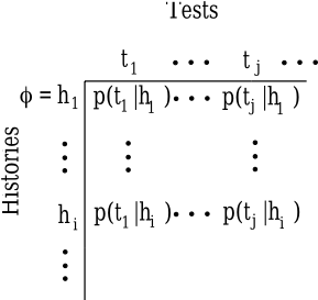
The theoretical development of mPSRs is best explained using the system dynamics matrix, D, that was developed in Singh et al. [2004]. The matrix D, shown in Figure 1, has all possible histories as rows and all possible tests as columns. The columns (rows) are arranged by test (history) length and within the same length in lexicographic ordering. The entry Dij = p(tj|hi) is the prediction for the j th test at the ith history. There is a one to one correspondence between system dynamics matrices and dynamical systems. The rank of D is the dimension of the corresponding dynamical system and is the number of core tests needed by the PSR model. The core tests of a PSR model correspond to a maximal set of linearly independent columns. Similarly, we can define a notion of core histories that correspond to a maximal set of linearly independent rows. We will only be interested in finite dimensional systems. This assumption is not terribly restrictive because all POMDPs with n underlying or nominal states are dynamical systems of dimension at most n. A full derivation of PSRs through use of the system dynamics matrix is presented in Singh et al. [2004].
memory-PSRs
The central idea behind mPSRs is to partition D into a set of m submatrices D1 . . .Dm by partitioning the set of histories (rows) but not the tests (columns), i.e., each submatrix Di contains all the columns but only a subset of the histories. How do memories enter this picture? We will use memory of past observations to partition histories, and every memory will correspond to a partition; we elaborate on this later. For now, note that each submatrix will have its own rank and its own core tests and core histories as well as model-update parameters. The set of memories and core tests for each partition form the basis of mPSR models. It is straightforward that the rank of each submatrix is at most the rank of the full matrix D. In the worst case, the ranks of all the submatrices are the same as the rank of D, in which case the resulting mPSR model may have (many) more parameters than the PSR model. But in other cases the ranks of the submatrices may be much smaller than the rank of D and then the resulting mPSR model may be more compact than the PSR model. We provide examples of both cases in Section 5. The size of the model is important because a model with fewer parameters should in general be more efficient (i.e., require less data) to learn. We also test this empirically in Section 5.
In this paper we do not address the question of automatically discovering useful ways of partitioning histories and instead assume that partitions correspond to history suffixes of some fixed length.
Definition of memory: For this paper, given an mPSR using length k suffixes, a memory is a specific sequence of length k that identifies a partition. So, when considering a history h and memories of length one, the memory at h is just the last (most recent) observation in h, and there will be |O| memories in the mPSR. For memories of length two, the memory at h is the last (most recent) action-observation pair in h, and there will be |A| ∗ |O| memories in the mPSR. In general, the set of possible memories in an mPSR that uses length-k suffixes is the set of all length-k sequences of alternating actions and observations that end in an observation; we will denote the size of such a set as mk.
Let µ1 . . . µmk represent all the distinct memories in an mPSR model. Also, let the memory at history h be denoted µ(h). Each memory µi has a corresponding submatrix Dµi created by the partition of histories corresponding to µi. The core tests for partition Dµ are referred to as µ-core tests to distinguish them from the core tests of the PSR model of the same system. Thus, the µ-core tests for the submatrices Dµ1 . . .Dµmk are denoted Qµ1 . . .Qµmk respectively. The prediction vector p(Qµ(h) |h) contains the predictions for the µ-core tests Qµ(h) at memory µh.
Definition of mPSR state: The mPSR state at history h is denoted by the concatenation of the memory at h and the prediction vector for that memory at h, i.e., as [µ(h), p(Qµ(h) |h)]. Thus, the mPSR state contains both a memory of the past as well as predictions about the future while a PSR state contains only predictions about the future.
Definition of mPSR update parameters: For each memory, µi, we will keep a set of matrices M µi ao and vectors mµi ao for all a, o. There is a subtle issue in defining these parameters. It is not the case that each submatrix is a separate dynamical system. Indeed if the memory corresponding to current history h is say µi and we take action a and observe o, the memory corresponding to the next history hao could be different from µi. Lets say it is µj. Thus the update parameters M µi ao must transform the current prediction vector that makes prediction for µ-core tests Qµi in history h to the prediction vector for µ-core tests Qµj in history hao. Note that all histories belonging to memory µi will transition to the same memory µj for action-observation pair ao, i.e., j is uniquely determined by i and the pair ao; and so the model parameter M µi ao need not explicitly reference to the next memory µj. Thus one can define the state update for mPSRs as follows: upon taking action a in history h and observing o
where µ(h) = µi and µ(hao) = µj. The matrix M µi ao is of size (|Qµi |×|Qµj |) and the vector mµi ao is of size (|Qµi |×1). As in PSRs the update parameters in mPSRs have meaning. For instance, the kth column of M µi ao is the (|Qµi | ×1)-sized constant parameter vector that computes the prediction for the test that is the kth µ-core test for memory µj.
The mPSR model parameters allow linear computation of the prediction for any test t = {a1o1 . . . akok} at history h as
where µ0 is the memory corresponding to history h, µ1 is the memory corresponding to history ha1o1 and so on.
Definition of mPSR: An mPSR model is defined by the tuple 〈A,O, µ1 . . . µmk ,Qµ1 . . .Qµmk ,M, [µ0, p(Qµ0 |∅)]〉 where A is the set of actions; O is the set of observations; µ1 . . . µmk are the possible memories; Qµi is the set of µcore tests for memory µi; M is the set of update parameters M µi ao and mµi ao for all a, o, µi; µ0 is the initial memory; and p(Qµ0 |∅) is the initial prediction vector.
A special and interesting case arises when a memory by itself serves as state and no predictions are needed.
Definition of landmark: Given an mPSR, a landmark is a memory that serves as state, i.e., is a sufficient statistic of history. Landmarks can be quite beneficial for making accurate predictions. We will discuss the identification of landmarks and exploiting them for prediction in Section 3.1.
3 Basic Theory of mPSRs
Our first result is to show that for any dynamical system it is possible to find µ-core tests for all memories in an mPSR model from the set Q of core tests for the corresponding PSR model.
Lemma 1. Let a dynamical system be modeled as a PSR with core tests Q. Then there always exists an mPSR model for the system such that for each memory µi the corresponding µcore tests Qµi satisfy Qµi ⊂ Q.
Proof. We provide a constructive proof which shows how to derive the subset Qµi from Q. Recall that all columns of D are linear combinations of the columns corresponding to Q in D. Consider the submatrix Dµi for memory µi. It must be the case that all columns of Dµi are linear combinations of the columns corresponding to Q in Dµi . Thus, there exists Qµi ⊂ Q.
In this paper, we don't exploit Lemma 1 for two reasons: 1) the core tests of PSRs are not unique, and 2) in any case when learning a model of a dynamical system from experience data we do not have a PSR model and thus its core tests Q to begin with.
Lemma 2. For any dynamical system of finite dimension and any choice of (fixed-length suffix) memories, the size of the resulting mPSR model for that system is at most the number of memories times the size of a PSR model for that system.
Proof. In the worst case, the rank of each of the submatrices in the mPSR is exactly the rank of the full system dynamics matrix. In such a case, if we happen to find different µ-core tests for each submatrix, then the model for each submatrix will be exactly as large as the PSR model.
The above lemma holds no matter how one chooses the memories. But what if we can choose the memories to use in constructing an mPSR judiciously (by which we mean to minimize the size of the resulting model)?
Theorem 1. With a judicious choice of memories, the size of the corresponding mPSR for any dynamical system is at least as compact as the size of the PSR for that dynamical system. Furthermore, there exist dynamical systems for which some choice of memories leads to an mPSR model that is more compact than the PSR model of the same dynamical system.
Proof. The proof of the first statement follows from the fact that a PSR is also an mPSR with the null set as memories. We prove the second statement by constructing such a dynamical system. Table 1 compares the size of mPSRs and PSRs for various standard test dynamical systems (based on POMDPs). In all instances, a suffix of length one was used to partition the histories. For at least three problems, Cheese, Shuttle and Four-Three, the mPSR is more compact than the PSR.
3.1 Landmarks
We show that landmarks are equivalent to memories for which there is only one µ-core test and furthermore that the prediction of any test at a landmark is the same at all histories that map to that landmark.
Lemma 3. For an mPSR model of a dynamical system,
- any memory that is a landmark has only one µ-core test, and every memory that has a µ-core set of size one is a landmark.
- for all histories that map to a landmark the prediction vector is a constant, i.e., independent of history.
- for all histories that map to a landmark the prediction of any test t is a constant, i.e., independent of history.
Proof. If µ is a landmark, then the predictions for all tests are fully determined when µ is known. Therefore, at any two histories that have memory µ, the prediction of every test is the same at both histories. This means that every row of Dµ must be identical, so the rank of Dµ is one, and only one µ-core test exists for µ.
For a memory µ that has a single µ-core test, qµ , let Hµ denote the histories that map to memory µ. For any h ∈ Hµ , and any action a, it must hold that ∑o p(ao|h) = 1 which implies that ∑o p(qµ |h)T mµao = 1, which in turn implies that p(qµ |h)T = 1/ ∑o mµao . Recall that mµao are independent of history, and thus the prediction of qµ must be independent of the history. This calculation exploits the fact that the prediction vector and update parameters are scalars.
| Problem | # Core Tests | # Param. Entries | ||
|---|---|---|---|---|
| PSR | mPSR | PSR | mPSR | |
| Tiger | 2 | 2,2 | 36 | 72 |
| Paint | 2 | 2,2 | 48 | 96 |
| Cheese | 11 | 1,1,1,1,2,2,3 | 3696 | 792 |
| Network | 7 | 4, 6 | 448 | 480 |
| Bridge | 5 | 2,2,4,4,5 | 1800 | 4488 |
| Shuttle | 7 | 1,1,2,2,4 | 840 | 450 |
| Four Three | 10 | 1,1,1,1,3,4 | 2640 | 748 |
| Float Reset | 5 | 1,5 | 120 | 96 |
Furthermore, because the prediction of qµ is independent of history, and the update vector mµt for any test t is independent of history, the prediction p(t|h) = p(qµ |h)T mµt of t at history h must also be independent of history. So, all rows of Dµ must be identical, and µ is therefore a landmark.
Landmarks come in handy because they can be used to keep a learned - and therefore only approximately correct -model from progressively drifting farther and farther away from reality as we make longer and longer term predictions from such a model. Every time we observe a landmark memory, we can reset the prediction vector to the constant corresponding to the landmark irrespective of the actual observed history. This can keep the error in the prediction for very long tests from growing with the length of the test. We exploit this ability in our empirical results below.
4 Learning mPSRmodels from data
In this section we present an algorithm for learning mPSR models from data under the assumption that the algorithm has the ability to reset the dynamical system being modeled to an initial state. We present the algorithm in two stages. In the first stage, we will assume that the algorithm has access to an oracle that if given a history h and test t will return the prediction p(t|h) for the dynamical system. In the second stage we will show how the oracle can be replaced by the use of sample data from the dynamical system with reset. Because we wish to minimize the amount of sample data needed by our algorithm, we will attempt to minimize the number of calls to the oracle in the first stage. Our algorithm is a relatively straightforward adaptation to mPSRs of the algorithm presented by James and Singh [2004] for PSRs.
4.1 Oracle based algorithm
Recall that there are two components to an mPSR: the µ-core tests for the different memories and the model-update parameters for the memories. In our empirical work below, we always use memories of length one. Clearly the model parameters for a memory depend on the choice of µ-core tests for that memory (recall that the µ-core tests are not unique). The process of computing µ-core tests and update parameters for each memory is identical and so we can just discuss how to do this for any one memory, say µi.
Determining µ-core tests and histories
The algorithm proceeds in iterations. At iteration t, the algorithm has a current set of linearly independent or µ-core tests and histories for each memory. Let Hµi t (T µi t ) be the set of µ-core histories (µ-core tests) found by iteration t for memory µi. These µ-core tests (histories) start off as the empty set at the first iteration. We also keep a set of candidate tests and histories at each iteration. The set of candidate tests for memory µi is the set of one-step tests; and for every ao pair, the set of ao-extensions for all the current µ-core tests for memory µj, where µj is the next memory when action a is taken in memory µi and o is observed. The set of candidate histories is similarly generated. We ask the oracle for the predictions of all the candidate tests at all the candidate histories. We compute the rank of this oracle-generated matrix, denoted Xt. The linearly independent rows and columns of Xt become the newHµi t+1 and T µi t+1 respectively. In selecting the new µ-core tests and histories we always include the previous µ-core tests and histories. We stop at iteration s if the rank of Xs is the same as the rank of Xs-1 for all memories.
The above algorithm is an adaptation of the similar algorithm for determining core test and histories for PSRs by James and Singh [2004]. Just like for PSRs this algorithm is not guaranteed to find all µ-core tests and histories, but also just like for PSRs it seems to work for all empirical work done so far.
Computing the model-update parameters
Now we discuss how to compute the model-update matrix M µ ao for any ao pair and any memory µ. We define a matrix A for memory µ that contains the predictions for all the µ-core tests at all the µ-core histories for memory µ. This matrix will have full rank and is computed in the algorithm above. Let µj be the memory achieved when action a is taken in memory µ and o is observed. The kth column of M µ ao , denoted x, is the constant parameter vector that computes the prediction for the ao-extension of the kth µ-core test, denoted y, of memory µj . Let b be the column vector of predictions of test y for the µcore histories of memory µ. We ask the oracle for the entries of b. Then from Equation 3 above, Ax = b. Since A is full rank, it is invertible and hence x = A-1 b. We can use the same idea to compute the model-update parameter vector mµao .
In the next section we show how the oracle needed for the above algorithm can be replaced by using data from the dynamical systemwith reset.
4.2 Learning mPSRs from sample data
We show how to obtain an estimate for the prediction p(t|h), something we went to the oracle for in the previous algorithm. We generate samples from the distribution p(t|h) by first taking the action sequence in h after a reset. If the observation sequence in h happens, then we have succeeded in generating history h. If we don't succeed in generating the history, we reset the system and try again. If we do succeed in generating the history, we take the action sequence in test t. If the observation sequence in test t happens, the test succeeds, else the test fails. We get an estimate of p(t|h) from the empirical success rate of the test t at history h. Of course, this is extremely wasteful in the number of data samples needed. We implement this basic idea much more efficiently by executing the action sequence in ht regardless of the observations obtained and then mining the data generated for all possible history and test pairs that can be extracted from it.
One problem that occurs with this estimation technique is that the sampled entries of the system dynamics matrix will almost certainly result in inaccurate calculations of rank (needed in the above oracle-based algorithm). We use a more robust rank calculation procedure developed in the PSR learning algorithm by James and Singh [2004]. The central idea is that we can use the number of samples that went into each entry of the matrix we wish to find the rank of to generate a threshold on singular values obtained via singular value decomposition. This threshold is more conservative when we have fewer samples and generally leads to a smaller rank than otherwise. As more samples are included, the threshold becomes less conservative and the calculated rank is closer to the straightforward calculation of rank.
5 Empirical results
We conducted experiments with a view towards validating four major ideas presented above. The first experiments are meant to compare the relative size of PSRs and mPSRs. The second is to test whether the oracle-based algorithm for computing mPSRs finds exact mPSR models. The third is to test the efficacy of the sample-data based learning algorithm for mPSRs. Finally, we are also interested in whether using landmarks, where available, to reset prediction vectors during the process of computing predictions for long test sequences provides a measurable benefit. All of these experiments were on a suite of standard POMDP-based dynamical systems [Cassandra, 1999] that have been used for both POMDP-learning as well for PSR-learning.
Again, for all of the results presented below, the memories used for the mPSR models were the most recent observation.
5.1 Comparing PSRs and mPSRs
For PSRs and mPSRs, the size of the model can be measured both in terms of the number of core tests (µ-core tests), and in the number of entries in the model parameters. Table 1 compares the sizes of PSR and mPSR models for the suite of test problems. For mPSRs, the number of µ-core tests at each memory is listed. Fully half of the test problems have landmarks (memories with only one µ-core test), indicating that this may be a fairly common situation.
The number of entries in the model parameters are listed for both PSRs and mPSRs. On three of the problems (Cheese, Shuttle, and Four-Three) there are significantly fewer entries needed for the mPSR model than for the PSR model; on three other problems (Tiger, Bridge, and Paint) there are significantly more; and on the two remaining problems there are approximately an equal number needed. This proves that mPSRs can be more compact than PSRs. This also illustrates that the unless we choose memories wisely, mPSRs can also be less compact than PSRs.
5.2 Constructing mPSRs from exact predictions
We tested the oracle algorithm for computing mPSRs by providing access to the true predictions computed analytically for the test problems. As we mentioned in Section 4.1, this algorithm is not guaranteed to find all µ-core tests for every memory. We found that in fact for all the test problems, the algorithm does indeed find all the µ-core tests and histories for all the models. We also verified that the resulting mPSR models were perfect, in the sense that any prediction error was due to machine round-off error. Furthermore, because correct sets of µ-core tests were discovered, all landmarks were identified.
5.3 Learning mPSRs from samples
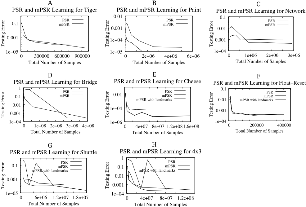
Here we present the results of learning mPSR models for all our dynamical systems. As mentioned above we assumed a reset. This makes our results directly comparable to the results of James and Singh [2004] on the same set of problems under the same reset assumption. We applied the algorithm of Section 4.2, stopping every so often during learning to test the model learned so far. For each test of the learned model, we asked the model to make predictions while tracking the system for 100, 000 steps (with randomly chosen actions). The test error reported is the average error in the one-step predictions of the model relative to the true predictions. This is the same error measure as used in James and Singh [2004].
The results of this testing are presented in Figure 2. We compare our results to the results for PSR learning for the same dynamical systems from James and Singh [2004]. Plots A to D present the results for the systems without any landmarks, and show the results of PSR and mPSR learning. In two of these systems, PSR learning is more efficient while in the other two they are roughly equivalent. We note that in all of these problems the PSR models are more compact or equal in size than the mPSR models. Plots E to H are for systems with landmarks. Here we plot three results: PSR learning, mPSR learning and mPSR learning with landmarks. The last algorithm, mPSR learning with landmarks, uses the mPSR learning algorithm of Section 4.2 but during testing resets the prediction vector when a landmark memory is encountered to the constant prediction for that memory. In three of the systems corresponding to graphs E, G and H, the size of the mPSR model is smaller than the PSR model. As we surmised in Section 2 this leads to mPSR learning being more efficient than PSR learning. In the system for plot F the two are roughly equivalent as are their sizes. The effect of using landmarks is most easily seen in plots G and H. Here mPSR learning without using landmarks is very noisy for if the system gets off-track in its predictions the error accumulates rapidly as the test sequence lengthens, while using the landmarks stabilizes the error and gives the best results.
6 Conclusion
In this paper we proposed a new class of models, mPSRs, that combines memory of past observations and predictions of future observations into its state representation. We showed that mPSRs are as expressive as and can be more compact than PSRs that solely use predictions of future observations in its state representation. Our preliminary empirical results showed that in dynamical systems where the mPSR model of the system is more compact than the PSR model, learning the mPSR model is more efficient than learning the PSR model. Finally, we formalized the notion of landmark memories and demonstrated how to find them and how to exploit them in making long-term predictions.
As future work, we will explore the interesting challenge of automatically finding good memories to combine with predictions of tests to make compact and efficiently learnable mPSR models.
Acknowledgements The research reported in this paper was supported by NSF grant IIS-0413004. The authors also thank Rich Sutton for helpful comments.
@inproceedings{ijcai2005p221,
  title     = {Combining Memory and Landmarks with Predictive State Representations},
  author    = {James, Michael R. and Wolfe, Britton and Singh, Satinder},
  booktitle = {Proceedings of the Nineteenth International Joint Conference on
               Artificial Intelligence, {IJCAI-05}},
  publisher = {International Joint Conferences on Artificial Intelligence},
  editor    = {Leslie Pack Kaelbling and Alessandro Saffiotti},
  pages     = {734--738},
  year      = {2005},
  url       = {https://ijcai.org/proceedings/2005/221},
}
TY - CPAPER TI - Combining Memory and Landmarks with Predictive State Representations AU - James, Michael R. AU - Wolfe, Britton AU - Singh, Satinder T2 - Proceedings of the Nineteenth International Joint Conference on Artificial Intelligence, IJCAI-05 PB - International Joint Conferences on Artificial Intelligence PY - 2005 SP - 734 EP - 738 UR - https://ijcai.org/proceedings/2005/221 ER -Copied
Machine-readable versions of this paper, for tools and AI agents:





