
Robust Planning with (L)RTDP
Proceedings of the Nineteenth International Joint Conference on Artificial Intelligence. Pages 1214-1218.
© 2005 International Joint Conferences on Artificial Intelligence
Abstract
Stochastic Shortest Path problems (SSPs), a subclass of Markov Decision Problems (MDPs), can be efficiently dealt with using Real-Time Dynamic Programming (RTDP). Yet, MDP models are often uncertain (obtained through statistics or guessing). The usual approach is robust planning: searching for the best policy under the worst model. This paper shows how RTDP can be made robust in the common case where transition probabilities are known to lie in a given interval.
- [Bagnell et al., 2001] J.A. Bagnell, A. Y. Ng, and J. Schnei- der. Solving uncertain markov decision problems. Technical Report CMU-RI-TR-01-25, Robotics Institute, Carnegie Mellon U., 2001.
- [Barto et al., 1995] A.G. Barto, S. Bradtke, and S. Singh. Learning to act using real-time dynamic programming. Ar- tificial Intelligence, 72, 1995.
- [Bertsekas and Tsitsiklis, 1996] D.P. Bertsekas and J.N. Tsitsiklis. Neurodynamic Programming. Athena Scien- tific, 1996.
- [Bonet and Geffner, 2003] B. Bonet and H. Geffner. Labeled rtdp: Improving the convergence of real time dynamic pro- gramming. In Proc. of the 13th Int. Conf. on Automated Planning and Scheduling (ICAPS'03), 2003.
- [Buffet and Aberdeen, 2004] O. Buffet and D. Aberdeen. Planning with robust (l)rtdp. Technical report, National ICT Australia, 2004.
- [Buffet, 2004] O. Buffet. Robust (l)rtdp: Reachability anal- ysis. Technical report, National ICT Australia, 2004.
- [Givan et al., 2000] R. Givan, S. Leach, and T. Dean. Bounded parameter markov decision processes. Artificial Intelligence, 122(1-2):71-109, 2000.
- [Hosaka et al., 2001] M. Hosaka, M. Horiguchi, and M. Ku- rano. Controlled markov set-chains under average cri- teria. Applied Mathematics and Computation, 120(1- 3):195-209, 2001.
- [Munos, 2001] R. Munos. Efficient resources allocation for markov decision processes. In Advances in Neural Infor- mation Processing Systems 13 (NIPS'01), 2001.
- [Nilim and Ghaoui, 2004] A. Nilim and L. El Ghaoui. Ro- bustness in markov decision problems with uncertain tran- sition matrices. In Advances in Neural Information Pro- cessing Systems 16 (NIPS'03), 2004.
- [Patek and Bertsekas, 1999] S. D. Patek and D. P. Bertsekas. Stochastic shortest path games. SIAM J. on Control and Optimization, 36:804-824, 1999.
- [Strehl and Littman, 2004] A. L. Strehl and M. L. Littman. An empirical evaluation of interval estimation for markov decision processes. In Proc. of the 16th Int. Conf. on Tools with Artificial Intelligence (ICTAI'04), 2004.
- [Sutton and Barto, 1998] R. Sutton and G. Barto. Reinforce- ment Learning: an introduction. Bradford Book, MIT Press, Cambridge, MA, 1998.
References were extracted automatically from the PDF and may contain errors.
Full text extracted automatically from the PDF; figures, tables and equations may differ. The PDF is the version of record.
1 Introduction
In decision-theoretic planning, Markov Decision Problems [Bertsekas and Tsitsiklis, 1996] are of major interest when a probabilistic model of the domain is available. A number of algorithms make it possible to find plans (policies) optimizing the expected long-term utility. Yet, optimal policy convergence results all depend on the assumption that the probabilistic model of the domain is accurate.
Unfortunately, a large number of MDP models are based on uncertain probabilities (and rewards). Many rely on statistical models of physical or natural systems, such as plant control or animal behavior analysis. These statistical models are sometimes based on simulations (themselves being mathematical models), observations of a real system or human expertise.
Working with uncertain models first requires answering two closely related questions: 1- how to model this uncertainty, and 2- how to use the resulting model. Existing work shows that uncertainty is sometimes represented as a set of possible models, each assigned a model probability [Munos, 2001]. The simplest example is a set of possible models that are assumed equally probable [Bagnell et al., 2001; Nilim and Ghaoui, 2004]. Rather than construct a possibly infinite set of models we represent model uncertainty by allowing each probability in a single model to lie in an interval [Givan et al., 2000; Hosaka et al., 2001].
Uncertain probabilities have been investigated in resource allocation problems [Munos, 2001] - investigating efficient exploration [Strehl and Littman, 2004] and state aggregation [Givan et al., 2000] - and policy robustness [Bagnell et al., 2001; Hosaka et al., 2001; Nilim and Ghaoui, 2004]. We focus on the later, considering a two-player game where the opponent chooses from the possible models to reduce the longterm utility.
Our principal aim is to develop an efficient planner for a common sub-class of MDPs for which some policies are guaranteed to eventually terminate in a goal state: Stochastic Shortest Path (SSP) problems. The greedy Real-Time Dynamic Programming algorithm (RTDP) [Barto et al., 1995] is particularly suitable for SSPs, as it finds good policies quickly and does not require complete exploration of the state space.
This paper shows that RTDP can be made robust. In Section 2, we present SSPs, RTDP and robustness. Then Sec. 3 explains how RTDP can be turned into a robust algorithm. Finally, experiments are presented to analyse the behavior of the algorithm, before a discussion and conclusion. 1
2 Background
2.1 Stochastic Shortest Path Problems
A Stochastic Shortest Path problem [Bertsekas and Tsitsiklis, 1996] is defined here as a tuple 〈S, s0,G,A, T, c〉. It describes a control problem where S is the finite set of states of the system, s0 ∈ S is a starting state, and G ⊆ S is a set of goal states. A is the finite set of possible actions a. Actions control transitions from one state s to another state s′ according to the system's probabilistic dynamics, described by the transition function T defined as T(s, a, s′ ) = Pr(st+1 = s′ |st = s, at = a). The aim is to optimize a performance measure based on the cost function c : S × A × S → R+. 2
SSPs assume a goal state is reachable from any state in S, at least for the optimal policy, so that one cannot get stuck in a looping subset of states. An algorithm solving an SSP has to find a policy that maps states to probability distributions over actions π : S → Π(A) which optimizes the long-term cost J defined as the expected sum of costs to a goal state.
In this paper, we only consider SSPs for planning purposes, with full knowledge of tuple defining the problem: 〈S, s0,G,A, T, c〉. In this framework, well-known stochastic dynamic programming algorithms such as Value Iteration (VI) make it possible to find a deterministic policy that corresponds to the minimal expected long-term cost J ∗ . Value Iteration works by computing the function J ∗ (s) that gives the expected sum of costs of the optimal policies. It is the unique solution of the fixed point Bellman equation:
1 Work presented in more details in [Buffet and Aberdeen, 2004]. 2 As the model is not certain, we do not make the usual assumption c(s, a) = Es′ [c(s, a, s′ )].
Updating J with this formula leads to asymptotic convergence to J ∗ . For convenience, we also introduce the Q-value: Q(s, a) = ∑s′∈S T (s, a, s′ )[c(s, a, s′ ) + V (s′ )].
SSPs can easily be viewed as shortest path problems where choosing a path only probabilistically leads you to the expected destination. They can represent a useful sub set of MDPs, as they are essentially finite-horizon MDPs with no discount factor.
2.2 RTDP
Trial based 3 Real-Time Dynamic Programming (RTDP), introduced in [Barto et al., 1995], uses the fact that the SSP costs are positive and the additional assumption that every trial will reach a goal state with probability 1. Thus, with a zero initialization of the long-term cost function J, both J and Q-values monotonically increase during their iterative computation.
The idea behind RTDP (Algorithm 1) is to follow paths from the start state s0, always greedily choosing actions with the lowest long-term cost and updating Q(s, a) as states s are encountered. In other words, the action chosen is the one expected to lead to the lowest future costs, until the iterative computations show that another action may do better.
Algorithm 1 RTDP algorithm for SSPs
RTDP(s:state) // s = s0 repeat RTDPTRIAL(s)
until // no termination condition RTDPTRIAL(s:state) while ¬GOAL(s) do a =GREEDYACTION(s) J(s)=QVALUE(s, a) s =PICKNEXTSTATE(s, a)
end while
RTDP has the advantage of quickly avoiding plans that lead to high costs. Thus, the exploration looks mainly at a promising subset of the state space. Yet, because it follows paths by simulating the system's dynamics, rare transitions are only rarely taken into account. The use of a simulation makes it possible to get good policies early, but at the expense of a slow convergence, because of the bad update frequency of rare transitions.
2.3 Robust Value Iteration
Pessimism and Optimism- We now turn to the problem of taking the model's uncertainty into account when looking for a "best" policy. The (possibly infinite) set of alternative models is denotedM.
3 We always assume a trial based RTDP implementation.
A simplistic approach computes the average model over M, or the most probable model inM, then uses standard SSP optimization methods. Such approaches guarantee nothing about the long-term cost of the policy if the true model differs from the one chosen for optimization.
We follow the approach described in [Bagnell et al., 2001], that consists of finding a policy that behaves well under the worst possible model. This amounts to considering a twoplayer zero-sum game where a player's gain is its opponent's loss. The player chooses a policy over actions while its "disturber" opponent simultaneously chooses a policy over models (as this is a simultaneous game, optimal policies can be stochastic). This results in a max-min-like algorithm:
In this SSP game, Value iteration does converge to a fixed solution [Patek and Bertsekas, 1999].
It is also possible to be optimistic, considering that both players collaborate (as they endure the same costs), which turns the max into a min in previous formula. This second case is equivalent to a classical SSP where a decision consists of choosing an action and a local model.
Locality - Such a max-min algorithm would be particularly expensive to implement. Even restricting the search to a deterministic policy over models, it requires computing the optimal long-term cost function for each model before picking the worst model found and the optimal policy associated with it. However, a simpler process may be used to compute J while looking simultaneously for the worst model. It requires the hypothesis that next-state distributions T(s, a, ·) are independent from one state-action pair (s, a) to another. This assumption does not always hold. However, this makes things easier for the opponent because it now has larger set of models from which to choose. This consequence is conservative for producing robust policies.
Because we assume independence at the state-action level (not only at the state level), it is equivalent to a situation where the second player makes a decision depending on the current state and the first player's action. This situation amounts to a sequential game where the previous players move is known to the next player: both players can act in a deterministic way without loss of efficiency.
The result of this assumption is that the worst model can be chosen locally when Q is updated for a given state-action pair. As can be seen from Algorithm 2, the worst local model mas may change while Q-values evolve. Previous updates of reachable states' long-term costs may change their relative ordering, changing which outcomes are considered to be worst.
The key contribution of this paper is to show that RTDP can be made robust, allowing for planning in very large and uncertain domains, retaining worst (or best) case behaviour guarantees.
3 Robust RTDP
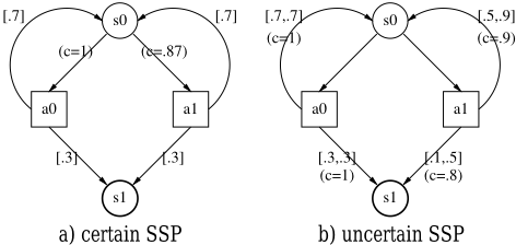
From now on, we consider interval-based uncertain SSPs, where T(s, a, s′ ) is known to be in an interval [Prmin (s′ |s, a), Prmax (s′ |s, a)]. Figure 1 is an example. We
Algorithm 2 Robust Value Iteration (for an SSP)
1: Initialize J to 0. 2: repeat 3: for all s: state do 4: for all a: action do 5: Qmax(s, a) ← maxmas ∈Mas ∑s′∈S Tmas (s, a, s′ ) [J(s′ ) + cmas (s, a, s′ )] 6: end for 7: J (i) ← mina∈A Qmax(s, a) 8: end for 9: until J convergesdiscuss the pessimistic approach, the optimistic one leading to similar results.
For a given state-action pair (s, a), there is a list R = (s′1 , · · · , s′k ) of reachable states. For each reachable state T(s, a, s′i ) ∈ Ii = [pmin i , pmax i ]. Thus, possible models are the ones that comply with these interval constraints while ensuring ∑i T(s, a, s′i ) = 1. Fig. 2 illustrates this with three reachable states.
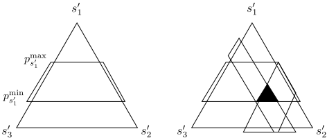
Worst LocalModels- Themaximisation step to compute Q(s, a) in Alg. 2 is done by giving the highest probability to the worst outcome. This requires firstly sorting reachable states in decreasing order of the values: c(s, a, s′1 )+J(s′1 ) ≥ c(s, a, s′2 )+J(s′2 ) ≥ · · · c(s, a, s′k )+J(s′k ). Then, the worst distribution is the one giving the highest probability to the first state s′1 , then to s′2 , and so on up to s′k . As pointed out in [Givan et al., 2000], this is equivalent to finding the highest index r ∈ [1..k] such that
The resulting transition probabilities are
Using the pre-computed bound Bmin = ∑ki=1 pmin i , Alg. 3 gives a complete implementation. The insertion sort algorithm 4 is chosen as the list will usually be ordered from previous J updates.
Algorithm 3 Worst Model for State-Action Pair (s, a)
WORSTMODEL(s: state, a: action)
end while
To summarise, Robust VI on an interval-based SSP consists of applying normal Value Iteration with the transition probabilities updated through Alg. 3.
We need only a single worst model to compute the corresponding Q-value. Yet, because several reachable states s′i may have the same value c(s, a, s′i )+J(s′i ) as s′r (we call this set of states S′r ), there may be an infinite number of equivalent worst local models. Any model differing only in how the probability mass is distributed among the equally bad states of S′r is also a worst local model.
Worst Global Models - Contrary to VI, RTDP does not necessarily visit the complete state-space. This is why [Barto et al., 1995] introduces the notion of relevant states, which we extend to the uncertain case: a state s is relevant for M if there exists a start state s0, a model m ∈ M and an optimal policy π under that model such that s can be reached from state s0 when the controller uses π under m.
4 http://en.wikipedia.org/wiki/Insertion sort
This notion is important because two equally worst local models on a given state-action pair may forbid different states, so that for two models m1 and m2, a state may be relevant in m1 but not in m2. Yet, RTDP should not find an optimal policy just for the relevant states of only one worst global model. Neither does the policy have to apply to all possible states. It should apply to all reachable states under any model (for optimal policies) i.e., for relevant states. But covering all relevant states in the worst model used for updating Q-values does not necessarily cover all relevant states inM: it depends on the model used to choose the next state, i.e., to simulate the system's dynamics.
To avoid missing relevant states, each local model used for the simulation should ensure that all reachable states can be visited. As can be seen in Fig. 2, the set of possible local models for a state-action pair is an n-dimensional convex polytope. Any model inside this polytope, excluding the boundary, is therefore adequate because, for all s′i , it ensures that P (s′i |s, a) > 0.
So there exists a global model md that can be used to effectively simulate the system's dynamics without missing any potentially reachable state.
3.1 Robust (Trial-Based) RTDP
Robust RTDP differs from the original RTDP in that:
- Each time the algorithm is updating a state's evaluation, an opponent is looking for a worst local model which serves to compute the Q-values.
- For exploration purposes, the algorithm follows dynamics of the system that consider all possible transitions (using model md).
- "Relevant" states are now the states reachable by following any optimal policy under any possible model.
From this, we adapt to our context convergence Theorem 3 from [Barto et al., 1995] and the corresponding proof, discussing mainly its changes.
Proposition 1. In uncertain undiscounted stochastic shortest path problems, robust Trial-Based RTDP with the initial state of each trial restricted to a set of start states, converges (with probability one) to J ∗ on the set of relevant states, and the controller's policy converges to an optimal policy (possibly nonstationary) on the set of relevant states, under the same conditions as Theorem 3 in [Barto et al., 1995].
Proof. The proof outline is:
- As shown in Sec. 2.3, robustness is achieved by considering a Stochastic Shortest Path Game (SSPG). In particular, this one is a sequential SSPG, for which Bertsekas and Tsitsiklis [1996] establish value iteration and Q-learning algorithms. Provided all states are visited infinitely often, asynchronous value iteration can also be used to solve sequential SSPGs (AVI-SSPG).
- We adapt the proof of Barto et al. [1995] to transform AVI-SSPG to an RTDP algorithm (RTDP-SSPG). The
- transformation ensures: 1- the additional maxm∈M in the update formula (Alg. 2, Line 5) does not break the requirement that Jt is increasing and non-overestimating; and 2- relevant states are visited infinitely often, guaranteeing a complete and optimal policy.
- RTDP-SSPG and robust RTDP differ because RTDPSSPG assumes an optimal opponent. In the robust case we wish to plan for opponents that may choose the wrong model. Thus robust RTDP is RTDP-SSPG following model md - for simulation only - that allows states to be visited that RTDP-SSPG optimal opponents would forbid. Under md (described in Sec. 3), no state reachable under any model in M is excluded from the search. Thus we have redefined an expanded set of relevant states for added robustness. All relevant states are still visited infinitely often.
Our use of the model md for simulation ensures that the policy will cover all states any opponent could lead us to, but assumes the worst model will apply afterwards.
4 Experiments
Labelled RTDP [Bonet and Geffner, 2003] is a modified version of RTDP which can be made robust in a similar way. The experiments conducted illustrate the behavior of robust LRTDP. To that end, it is compared to Bagnell et al.'s Robust Value Iteration, as well as LRTDP. In all cases, the convergence criteria is ϵ = 10-3 for LRTDP, and for VI we stop when the maximum change in a state long-term cost over one iteration is less than 10-3 .
4.1 Heart
In this first experiment, we compare a non-robust optimal policy with a robust one on the small example of Fig. 1-b. Table 1 shows the theoretical expected long-term costs of each policy on the normal (most probable) model, as well as the pessimistic and optimistic ones. The robust policy is largely better in the pessimistic case.
| Normal | Pessimistic | Optimistic | |
|---|---|---|---|
| Non-robust | 2.90 | 8.90 | 1.70 |
| Robust | 3.33 | 3.33 | 3.33 |
4.2 Mountain-Car
We use here the mountain-car problem as defined in [Sutton and Barto, 1998]: starting from the bottom of a valley, a car has to get enough momentum to reach the top of a mountain (see Fig. 3). The same dynamics as described in the mountain car software 5 have been employed. The objective is to minimize the number of time steps to reach goal.
5 http://www.cs.ualberta.ca/˜sutton/· · · MountainCar/MountainCar.html
-1.2
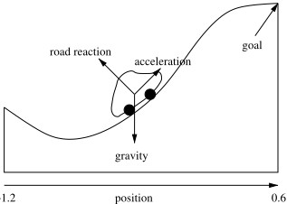
The continuous state-space is discretized (32 × 32 grid) and the corresponding uncertain model of transitions is obtained by sampling 1000 transitions from each state-action pair (s, a). For each transition, we computed intervals in which the true model lies with 95% confidence.
Results- Preliminary remark: simulating a path generally shows a car oscillating several times before leaving the valley. This has two main explanations: 1- the speed gathering is just sufficient to reach the summit, but not over it; and 2- the discretized model is not accurate enough and applying the policy obtained on the true mathematical model (instead of the discretized one) should be much better.
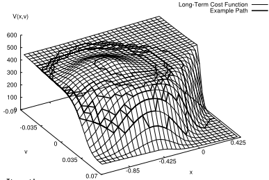
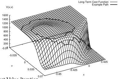
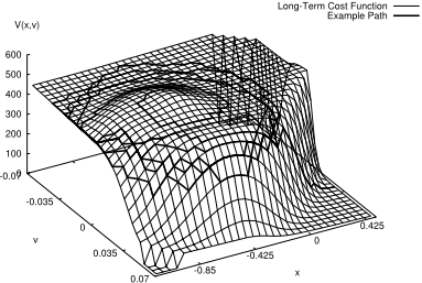
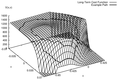
Fig. 4 shows the long-term cost function obtained by using value iteration, LRTDP, and their robust counterparts on the mountain-car problem. The x and y axes are the car's position and speed. The z axis is the expected cost to the goal. On the surface is an example path from the start state to a goal state: it follows the greedy policy under the average model.
The general shape of the surface obtained is always the same, with some unexplored parts of the state-space in LRTDP and Robust LRTDP (as expected). The vertical scales are much larger in robust cases. This reflects the fact that reaching the goal is much more time-consuming under a pessimistic model. Because J can here be interpreted as the average time to the goal, these graphs show how a small uncertainty can lead to longer policies. Here the times are multiplied by more than 2.5.
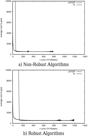
While executing the four different algorithms, an evaluation of the current greedy policy was made every 10 ∗ nStates = 10240 Q-value updates. The result appears in Fig. 5, the y axis being the expected cost to the goal from the start state. On both sub-figures, LRTDP-based algorithms obtain good policies quickly, but have slow convergence times of VI=2.83 × 10⁶ updates, LRTDP=6.76 × 10⁶ , rVI=8.31×10⁶ , rLRTDP=11.06×10⁶ .
Other experiments [Buffet and Aberdeen, 2004] also confirm these results, with one example showing that LRTDP can have a faster convergence than VI, and another one illustrating this approach on a temporal planning problem.
5 Discussion and Conclusion
A simple extension to this work, suggested by Hosaka et al. [2001], is to find the set of worst models as we do in this
a) Value Iteration
b) Robust Value Iteration
c) LRTDP
d) Robust LRTDP
Figure 4: Long-term cost functions for the mountain-car problem. In each case, an example path is generated based on the most likely model.
paper, but then to choose from these the model that has the lowest cost under an optimistic model. This improvement is presented in [Buffet and Aberdeen, 2004].
The approach to robustness adopted in this paper considers the knowledge of a set of possible models. An open question is whether it is possible to use more information from our uncertain model, by taking the probability distribution over possible models into account.
Model uncertainty has similarly been considered in model learning while planning [Strehl and Littman, 2004]. The algorithm proposed is optimistic, but does not seem to adapt well to our framework as an evolving model can break the "no-overestimation" assumption: ∀s ∈ S, t ≥ 0, Jt(s) ≤ J ∗ (s). It is still important to notice that robust RTDP would not suffer on-line, as the real dynamics can be employed to pick a next state (the worst model appearing only in the longterm cost update formula).
Finally, a crucial assumption in RTDP is that a goal state must be reachable from any state. We present an algorithm tackling this problem in [Buffet, 2004].
Conclusion - Recent works show that model uncertainty is a major issue in decision-theoretic planning. We have proposed a modification of the RTDP algorithm enabling it to compute robust policies efficiently in large and uncertain domains. Model uncertainty is represented through confidence intervals on transition probabilities. The convergence of the resulting algorithm is sketched. We demonstrate robust LRTDP on a domain where statistics are used to estimate appropriate intervals.
Acknowledgments
National ICT Australia is funded by the Australian Government. This work was also supported by the Australian Defence Science and Technology Organisation.
@inproceedings{ijcai2005p219,
  title     = {Robust Planning with (L)RTDP},
  author    = {Buffet, Olivier and Aberdeen, Douglas},
  booktitle = {Proceedings of the Nineteenth International Joint Conference on
               Artificial Intelligence, {IJCAI-05}},
  publisher = {International Joint Conferences on Artificial Intelligence},
  editor    = {Leslie Pack Kaelbling and Alessandro Saffiotti},
  pages     = {1214--1218},
  year      = {2005},
  url       = {https://ijcai.org/proceedings/2005/219},
}
TY - CPAPER TI - Robust Planning with (L)RTDP AU - Buffet, Olivier AU - Aberdeen, Douglas T2 - Proceedings of the Nineteenth International Joint Conference on Artificial Intelligence, IJCAI-05 PB - International Joint Conferences on Artificial Intelligence PY - 2005 SP - 1214 EP - 1218 UR - https://ijcai.org/proceedings/2005/219 ER -Copied
Machine-readable versions of this paper, for tools and AI agents:





