
Location-Based Activity Recognition using Relational Markov Networks
Proceedings of the Nineteenth International Joint Conference on Artificial Intelligence. Pages 773-777.
© 2005 International Joint Conferences on Artificial Intelligence
Abstract
In this paper we define a general framework for activity recognition by building upon and extending Relational Markov Networks. Using the example of activity recognition from location data, we show that our model can represent a variety of features including temporal information such as time of day, spatial information extracted from geographic databases, and global constraints such as the number of homes or workplaces of a person. We develop an efficient inference and learning technique based on MCMC. Using GPS location data collected by multiple people we show that the technique can accurately label a person’s activity locations. Furthermore, we show that it is possible to learn good models from less data by using priors extracted from other people’s data.
- [Ashbrook and Starner, 2003] D. Ashbrook and T. Starner. Using GPS to learn significant locations and predict movement across multiple users. In Personal and Ubiquitous Computing, 2003.
- [Geyer and Thompson, 1992] C. J. Geyer and E. A. Thompson. Constrained Monte Carlo Maximum Likelihood for dependent data. Journal of Royal Statistical Society, 1992.
- [Gilks et al., 1996] W.R. Gilks, S. Richardson, and D.J. Spiegel- halter. Markov Chain Monte Carlo in Practice. Chapman and Hall/CRC, 1996.
- [Hariharan and Toyama, 2004] R. Hariharan and K. Toyama. Project Lachesis: parsing and modeling location histories. In Geographic Information Science, 2004.
- [Hariharan et al., 2005] R. Hariharan, J. Krumm, and E. Horvitz. Web-enhanced GPS. In International Workshop on Location- and Context-Awareness, 2005.
- [Kumar and Hebert, 2003] S. Kumar and M. Hebert. Discrimina- tive random fields: A discriminative framework for contextual interaction in classification. In Proc. of the International Confer- ence on Computer Vision (ICCV), 2003.
- [Lafferty et al., 2001] J. Lafferty, A. McCallum, and F. Pereira. Conditional random fields: Probabilistic models for segmenting and labeling sequence data. In Proc. of the International Confer- ence on Machine Learning (ICML), 2001.
- [Liao et al., 2004] L. Liao, D. Fox, and H. Kautz. Learning and inferring transportation routines. In Proc. of the National Con- ference on Artificial Intelligence (AAAI), 2004.
- [Peng and McCallum, 2004] F. Peng and A. McCallum. Accurate information extraction from research papers using conditional random fields. In HLT-NAACL, 2004.
- [Philipose et al., 2004] M. Philipose, K.P. Fishkin, M. Perkowitz, D.J. Patterson, D. Hhnel, D. Fox, and H. Kautz. Inferring ADLs from interactions with objects. IEEE Pervasive Computing, 3(4), 2004.
- [Salazar et al., 2000] A. Salazar, D. Warden, K. Schwab, J. Spec- tor, S. Braverman, J. Walter, R. Cole, M. Rosner, E. Martin, and R. Ellenbogen. Cognitive rehabilitation for traumatic brain in- jury. Journal of American Medical Association, 283(23), 2000.
- [Sha and Pereira, 2003] Fei Sha and Fernando Pereira. Shallow parsing with conditional random fields. In Proceedings of Hu- man Language Technology-NAACL, 2003.
- [Taskar et al., 2002] B. Taskar, P. Abbeel, and D. Koller. Discrim- inative probabilistic models for relational data. In Proc. of the Conference on Uncertainty in Artificial Intelligence (UAI), 2002.
References were extracted automatically from the PDF and may contain errors.
Full text extracted automatically from the PDF; figures, tables and equations may differ. The PDF is the version of record.
1 Introduction
Activity recognition and context-aware computing are gaining increasing interest in the AI and ubiquitous computing communities. Most existing systems have been focused on relatively low level activities within small environments or during short periods of time. In this paper, we describe a system that can recognize high level activities (e.g., working, shopping, and dining out) over many weeks. Our system uses data from a wearable GPS location sensor, and is able to identify a user's significant places, and learn to discriminate between the activities performed at these locations - including novel locations. Such activity information can be used in many applications. For example, it could be used to automatically instruct a user's cell phone not to ring when dining at a restaurant, or it could support home rehabilitation of people suffering from traumatic brain injuries [Salazar et al., 2000] by providing automatic activity monitoring. Beyond estimating high-level activity categories, our system can be expanded to incorporate additional sensor information, thereby recognizing fine-grained indoor household tasks, such as those described in [Philipose et al., 2004].
Because behavior patterns can be highly variable, a reliable discrimination between activities must take several sources of evidence into account. Our system considers (1) temporal information such as time of day; (2) spatial information extracted from geographic databases, including information about the kinds of businesses in various locations; (3) sequential information such as which activity follows which activity; and (4) global constraints such as the number of different homes or workplaces. Additionally, it uses data collected by other users so as to improve the classification of a specific user's activities. All these constraints are soft: for example, on some days a person may do something unusual, such as go to a movie in the middle of a workday. Furthermore, the norm for some individuals may be different than our general commonsense prior: for example, some people work two jobs, or shuttle between two different homes. It is necessary to use a rich and flexible language to robustly integrate such a wide variety of both local and global probabilistic constraints.
Our system builds upon previous work on extracting places from traces of users' movements, gathered by GPS or other localization technologies [Ashbrook and Starner, 2003; Hariharan and Toyama, 2004; Liao et al., 2004]. Our work goes beyond theirs in that our system also recognizes the activities associated with the places. Moreover, previous approaches to modeling personal movements and place patterns require a large amount of training data from each user, and cannot be generalized to new places or new users. By contrast, our relational approach requires less individual training data by leveraging data collected by others. In summary, the contributions of this paper are:
- A general framework for sensor-based activity recognition based on Relational Markov Networks (RMNs) [Taskar et al., 2002], which are both highly expressive and well-suited for discriminative learning;
- An extension of RMNs to incorporate complex, global features using aggregations and label-specific cliques;
- Efficient Markov-chain Monte-Carlo (MCMC) algorithms for inference and learning in extended RMNs, and in particular, an MCMC algorithm to simultaneously evaluate a likelihood function and its gradient;
- Positive experimental results on real data from multiple subjects, including evidence that we can improve accuracy by extracting priors from others' data.
This paper is organized as follows. We will introduce our relational activity model in Section 2. Inference and learning will be discussed in Section 3, followed by experimental evaluations. Conclusions and future work are given in Section 5.
2 The Relational ActivityModel
In this section we first discuss RMNs and our extensions. Then we show how to use them for modeling activities.
2.1 Relational Markov Networks
RMNs are extensions of Conditional Random Fields (CRFs), which are undirected graphical models that were developed for labeling sequence data [Lafferty et al., 2001]. CRFs are discriminative models that have been shown to out-perform generative approaches such as HMMs and Markov random fields in areas such as natural language processing [Lafferty et al., 2001] and computer vision [Kumar and Hebert, 2003]. RMNs extend CRFs by providing a relational language for describing clique structures and enforcing parameter sharing at the template level. Thereby RMNs are an extremely flexible and concise framework for defining features that can be used in the activity recognition context.
An RMN consists of three parts: a schema E for the domain, a set of relational clique templates C, and corresponding potentials Φ. The schema E specifies the set of classes (i.e., entity types) and attributes in each class. An attribute could be a content attribute, a label attribute, or a reference attribute that specifies reference relation among the classes. An instantiation I of a schema specifies the set of entities for each class and the values of all attributes for each entity. In our context an instantiation consists of the sequence of all significant locations visited by a user along with the temporal and spatial attributes.
A relational clique template C ∈ C is similar to a relational database query (e.g., SQL) in that it selects tuples from an instantiation I; the query result is denoted as C(I). We extend the definition of such templates in two ways. First, we allow a template to select aggregations of tuples. For example, we can group tuples and define potentials over counts or other statistics of the groups. Second, we introduce label-specific cliques, whose structures depend on values of the labels. For example, our model can construct a clique over all activities labeled as "AtHome." Because labels are hidden during inference, such cliques potentially involve all the labels. Labelspecific cliques can be specified by allowing label attributes to be used in the "Where" clause of an SQL query.
Each clique template C is associated with a potential function φC(vC) that maps a tuple (values of variables or aggregations) to a non-negative real number. Using a log-linear combination of feature functions, we get the following representation: φC(vC) = exp{wTC · fC(vC)}, where fC() defines a feature vector for C and wTC is the transpose of the corresponding weight vector. For instance, a feature could be the number of different homes defined using aggregations.
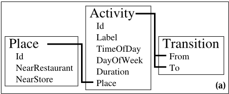
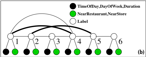
For a specific instantiation I, an RMN defines a conditional distribution p(y|x) over labels y given the observed attributes x. To compute such a conditional distribution, the RMN generates an unrolled Markov network, in which the nodes correspond to the content attributes and the label attributes. The cliques of the unrolled network are built by applying each clique template C ∈ C to the instantiation, which can result in several cliques per template (see Fig. 1(b) for an example). All cliques that originate from the same template must share the same weights wC. The resulting cliques factorize the conditional distribution as
where the normalizing partition function Z(x) = ∑y′ ∏C∈C ∏v′C ∈C φC(v′C ). (3) follows by moving the products into the exponent and combining all summations into w and f .
2.2 Relational ActivityModels
We will now describe our relational activity models. Even though we illustrate the concepts using the example of location-based activity recognition, our model is very flexible and can be applied to a variety of activity recognition tasks.
The schema for activity recognition based on temporal and spatial patterns is shown in Fig. 1(a). It includes three classes: Activity, Place, and Transition.
Activity: Activity is the central class in the domain. Its attribute Label is the only hidden variable. The set of possible labels in our experiments is {'AtHome', 'AtWork', 'Shopping', 'DiningOut', 'Visiting', 'Others'}. Attribute Id serves as the primary key. The class also contains temporal information associated with an activity, such as TimeOfDay, DayOfWeek, and Duration, whose values are discretized when necessary. Finally, Place is a reference attribute that points to a Place entity where the activity has been performed.
Place: The class Place includes two boolean attributes: NearRestaurant and NearStore, which indicate whether there are restaurants or stores nearby.
Transition: Transition captures temporal succession relationship among activities. The reference attributes From and To refer to a pair of consecutive activities.
Based on the schema, we define the following relational clique templates. Each of them takes into account a number of discriminative features.
- Temporal patterns: Different activities often have different temporal patterns, such as their duration or time of day. Such local patterns are modeled by clique templates that connect each attribute with the activity label.
- Geographic evidence: Information about the types of businesses close to a location can be extremely useful to determine a user's activity. Such information can be extracted from geographic databases, such as Microsoft MapPoint [Hariharan et al., 2005] used in our experiments. Since location information in such databases is not accurate enough, we consider such information by checking whether, for example, a restaurant is within a certain range from the location.
- Transition relations: The first-order transitions between activities can also be informative. For example, staying at home followed by being at work is very common
while dining out immediately followed by another dining out is rare. The SQL query for this clique template is:
SELECT a1.Label, a2.Label FROM Activity a1, Activity a2, Transition t WHERE t.From=a1.Id AND t.To=a2.Id
- Spatial constraints: Activities at the same place are often similar. In other words, the number of different types of activities in a place is often limited. We can express such a constraint using an aggregation function Count():
SELECT COUNT(DISTINCT Label)
FROM Activity
GROUP BY Place
- Global features: Such features model global, soft constraints on activities of a person. The number of different home locations is an example of global constraints. Such a constraint is modeled by a clique template that selects all places labeled as home and returns how many of them are different:
SELECT COUNT(DISTINCT Place)
FROM Activity
WHERE Label='AtHome'
Note that the label variable appears in the "Where" clause, so this is an example of label-specific clique. In a different activity recognition context, global features could also model information such as "the number of times a person has lunch per day."
In the first three templates, the feature functions fC() are just indicator functions that return binary values. They can also return numbers, such as in the last two templates.
3 Inference and Learning
3.1 Labeling Activities
In our application, the task of inference is to estimate the labels of activities given a sequence of locations visited by a person. To do so, our RMN converts a location sequence into unrolled Markov networks, as illustrated in Fig. 1(b). Inference in our relational activity model is complicated by the fact that the structure of the unrolled Markov network can change during inference because of the label-specific cliques. Using standard belief propagation in such networks would require the construction of cliques over all labels, which is obviously inefficient [Taskar et al., 2002]. We overcome this problem by using MCMC for inference [Gilks et al., 1996]. In a nutshell, whenever the label of an object is changed during sampling, we determine all cliques that could be affected by this change and re-compute their potentials.
We first implemented MCMC using basic Gibbs sampling. Unfortunately, this technique performs poorly in our model because of the strong dependencies among labels. To make MCMC mix faster, we first make an additional spatial constraint that all activities occurring in the same place must have the same label (the relaxation of this constraint will be addressed in future work). This hard constraint allows us to put all activities occurring in the same place into a so-called block. We then develop a mixture of two transition kernels that converges to the correct posterior.
The first kernel is a block Gibbs sampler. At each step we update the labels in a block simultaneously by sampling from the full conditional distribution
where k is the index of the block, yk is the label of block k, y-k are the labels for blocks other than k. The second kernel is a Metropolis-Hasting (MH) sampler. To update the label for block k, the MH sampler randomly picks a block j and proposes to exchange label yk and yj. The acceptance rate of the proposal follows as
where y and y′ are the labels before and after the exchange, respectively.
The numbers of different homes and workplaces are stored in the chains as global variables. This allows us to compute the global features locally in both kernels: in the Gibbs kernel we increase or decrease the numbers depending on the labels of the given block and in the MH kernel the numbers remain intact. At each time step, we choose the Gibbs sampler with probability γ, and the MH sampler with probability 1 - γ.
3.2 Supervised Learning
We show how to learn generic activity models from labeled activity sequences of N different users. Learning a customized model for an individual user is a special case when N = 1. The parameters to be learned are the feature weights w that define clique potentials in (3). To avoid overfitting, we perform maximum a posterior (MAP) parameter estimation and impose an independent Gaussian prior with constant variance for each component of w, i.e., p(w) ∝ exp{-(wµ)T · (w-µ)/2σ2 }, where µ is the mean and σ2 is the variance . We define the MAP objective function as the negative log-likelihood of training data from N subjects plus the prior:
where j ranges over different users and yj are the activity labels for each user. Since (6) is convex, the global minimum can be found using standard optimization algorithms [Taskar et al., 2002]. We apply the quasi-Newton technique to find the optimal weights [Sha and Pereira, 2003]. Each iteration of this technique requires the value and gradient of (6) computed at the weights returned in the previous iteration.
Evaluating the objective function
It can be intractable to compute exact objective values in (6) for all but the simplest cases. This is due to the fact that, for a specific w, it is necessary to evaluate the partition function Z(xj , w), which requires summation over all possible label configurations. We approximate the objective value using Monte-Carlo methods [Geyer and Thompson, 1992]. Suppose we already know the value of L( ˜w) for a weight vector ˜w. Then for each subject j, we use our MCMC inference to get M random samples, ˜y(i) j (1 ≤ i ≤ M), from the distribution P(y | xj, ˜w). Then L(w) can be approximated as:
where ∆˜f (i) j = f(xj, ˜y(i) j ) - f(xj, yj) is the difference between sampled feature counts using ˜w and the empirical feature counts in the labeled data.
Eq. (7) can only be used to estimate values of L(w) relative to L( ˜w). Fortunately, such relative values are sufficient for the purpose of optimization. It can be shown that the best approximation in (7) is obtained when ˜w is close to the optimal w. Therefore, during optimization, our algorithm updates ˜w with better weight estimates whenever possible.
Evaluating the gradient
The gradient of the objective function, ∇L(w), equals to the difference between the sampled feature counts and the empirical feature counts, plus a prior term. To generate the sampled feature counts under w, we again run MCMC inference. Suppose we have obtained M random samples, y(i) j (1 ≤ i ≤ M), from the distribution P(y | xj,w). We can compute the gradient as:
input : the weights w provided by the optimizer output: L(w) and ∇L(w) //Evaluate the gradient ∇L(w) foreach subject j do Run MCMC with w and get M samples; Get feature count difference ∆f (i) j (1 ≤ i ≤M) ; end Compute the gradient ∇L(w) using Eq. (8) ; //Evaluate the objective value L(w) if First time calling this function then L( ˜w) = L(w) = 0; ˜w =w ; ∆˜f (i) j =∆f (i) j for 1 ≤ j ≤ N,1 ≤ i ≤M ; else Compute L(w) using Eq. (7) ; if L(w) < L( ˜w) then L( ˜w) = L(w); ˜w =w ; ∆˜f (i) j =∆f (i) j for 1 ≤ j ≤ N,1 ≤ i ≤M ; end endwhere ∆f (i) j = f(xj, y(i) j ) - f(xj, yj) is the difference between the sampled and the empirical feature counts.
Algorithm
If we compare (7) and (8), we see both require the difference between the sampled and the empirical feature counts. While samples in (7) are based on the weights ˜w, those in (8) are based on w. Therefore, if we always keep the best weight estimate as ˜w, we can reuse the sampled feature counts from gradient estimation, thereby making objective value evaluation very efficient.
Our algorithm simultaneously estimates at each iteration the value and the gradient of the negative log-likelihood (6) for given weights w. These estimates are used by the quasiNewton approach to compute new weights, and then the estimation is repeated. As shown in Alg. 1, both L( ˜w) and L(w) are initialized as 0 and thus all the objective values are evaluated relative to the objective value of initial weights. In later iterations, when we find a better weight estimate that makes L(w) less than L( ˜w), we update ˜w with the new w and also keep the new L( ˜w) and ∆˜f (i) j (1 ≤ j ≤ N, 1 ≤ i ≤ M). By doing that, we not only evaluate objective values very efficiently, but are also able to get more accurate approximations as ˜w approaches closer to the optimal weights.
4 Experiments
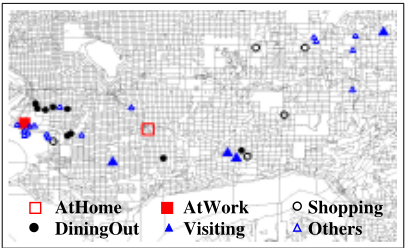
To evaluate our location-based activity recognition technique, we collected two sets of location data using wearable GPS units. The first data set (called "single") contains location traces from a single person over a time period of four months (see Fig. 2). It includes about 400 visits to 50 different places. The second data set (called "multiple") was collected by five different people, about one week for each. Each person's data include 25 to 35 visits and 10 to 15 different places. We extracted places / visits from the GPS logs by detecting locations at which a person spends more than 10 minutes [Hariharan and Toyama, 2004]. Each instance corresponds to an activity. We then clustered nearby activity locations into places. For training and evaluation, we let the subjects manually label the types of activities. Then, we trained the models and tested their accuracy. Accuracy was determined by the activities for which the most likely labeling was correct.
Applying learned models to other people
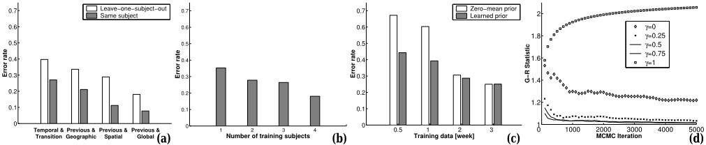
In practice, it is of great value to learn a generic activity model that can be immediately applied to new users without additional training. In this experiment, we used the "multiple" data set and performed leave-one-subject-out crossvalidation: we trained using data from four subjects, and tested on the remaining one. The average error rates are indicated by the white bars in Fig. 3(a). By using all the features, the generic models achieved an average error rate of 18%. It can be seen that global features and spatial constraints significantly improve classification. To gage the impact of different habits on the results, we also performed the same evaluation using the "single" data set. In this case, we used one-month data for training and the other three-month data for test, and we repeated the validation process for each month. The results are shown by the gray bars in Fig. 3(a). In this case, the models achieved an error rate of only 7% by using all the features. This experiment shows that it is possible to learn good activity models from groups of people. It also demonstrates that models learned from more "similar" people can achieve higher accuracy. This indicates that models can be improved by grouping people based on their activity patterns.
Table 1 shows the confusion matrix of one experiment on generic models (rightmost white bar in Fig. 3(a)). As can be seen, our approach is able to perfectly label homes and workplaces. The technique performs surprisingly well on the other activities, given that they are extremely difficult to distinguish based on location information alone. The confusion matrix also shows that simply labeling places by the most frequent activity (home) would result in an error rate of 62%.
| Inferred labels | ||||||
|---|---|---|---|---|---|---|
| Truth | Home | Work | Shop | Dining | Visit | Other |
| Home | 57 | 0 | 0 | 0 | 0 | 0 |
| Work | 0 | 34 | 0 | 0 | 0 | 0 |
| Shop | 0 | 0 | 8 | 2 | 0 | 4 |
| Dining | 0 | 0 | 3 | 6 | 0 | 4 |
| Visit | 0 | 0 | 1 | 0 | 4 | 3 |
| Other | 0 | 0 | 6 | 1 | 2 | 15 |
To evaluate the impact of number of people available for model learning, we trained our model using data from different numbers of subjects and tested on the remaining one (all features were used). The average error rates of the crossvalidation are shown in Fig. 3(b). When trained using only one subject, the system does not perform well (error rate of 35%), mainly because many patterns specific to that person are applied onto others. When more subjects are used for training, the patterns being learned are more generic and the models achieve significantly higher accuracy.
Improved learning through priors extracted from others
When estimating the weights of RMNs, a prior is imposed in order to avoid overfitting. Without additional information, a zero mean Gaussian is typically used as the prior [Taskar et al., 2002]. [Peng and McCallum, 2004] demonstrated that better accuracy can been achieved if feature-dependent variances are used. Our experiment shows that performance can also be improved by estimating the prior means of the weights (µ in Eq. (6)) using data collected from other people.
In this experiment, we compared the models of a specific person trained using a zero-mean prior with the models trained using an estimated prior. In the latter case, we first learned the feature weights from other people and used those as the mean of the Gaussian prior. We evaluated the performance for different amounts of training data available for the test person. The results are shown in Fig. 3(c), in which the error rates are counted only on the novel places, i.e., places that were not visited in the training data and thus often very irregular. We can see that using data from others to generate a prior boosts the accuracy significantly, especially when only small amounts of training data are available.
The Bayesian prior allows the model to smoothly shift from generic to customized: On one end, when no data from the given subject are available, the approach returns the generic (prior) model; on the other end, as more labeled data become available, the model adjusts more and more to the specific patterns of the user.
Additional experiments
For comparison, we also built basic HMMs in which the hidden states are the labels and all the observations are independent given the states. Parameter estimation in HMMs with labeled data is done via frequency counting. The most likely labels can be found using the Viterbi algorithm. In the one-month-training cross-validation on the "single" data set, the HMM produced an average error rate of 21.1% by using the temporal, geographic, and transition features. 1 Because of the advantages of discriminative learning, even using the same features, RMNs performed better than HMMs and reduced the relative error rate by about 10%.
In a separate set of experiments, we tested the performance of our MCMC sampler. By visualizing the standard GelmanRubin statistics [Gilks et al., 1996] generated from parallel chains, we observed that by combining the Gibbs and the MH kernels, MCMC converged much faster than using only one of them (see Fig. 3(d)). All results reported here were achieved with a mixing parameter γ = 0.5 (see Section 3).
1 Spatial constraints and global features do not satisfy the firstorder Markov assumption and thus are difficult to model as HMMs.
5 Conclusions and FutureWork
In this paper, we presented a discriminative relational approach for activity recognition based on the framework of RMNs, which are well-suited to model constraints for activity recognition. We showed how to perform efficient inference and learning using MCMC with a mixture of kernels.
Using our relational approach, we developed and tested a specific model for location-based activity recognition. The results are very promising: the system is able to learn models that can accurately label human activities solely based on GPS data. We demonstrated that spatial and global features are very important to achieve good recognition rates. We also showed how to obtain good priors using data from other people so as to learn an improved model for a specific person that requires less labeled data.
We plan to extend our model in a number of ways. First, by collecting data from more subjects, we can learn a set of generic models by clustering the subjects based on their similarities; then we can use a mixture of these models to better recognize activities of a new person. Second, we will relax the hard spatial constraint of one activity per location and thus recognize different activities performed at the same place. Third, we will integrate information from other wearable sensors (e.g., microphones or accelerometers) into our general framework, thereby enabling much finer-grained activity recognition. We will also apply the model to the problem of estimating a person's indoor activities from RFID sensor data. By incorporating constraints such as "a person typically has lunch once per day," we expect strong improvements over the results reported in [Philipose et al., 2004].
Acknowledgments
We thank Anthony LaMarca, Don J. Patterson, and Xiaolin Sun for collecting data used in our experiments. We would also like to thank John Krumm for suggesting the use of geographic databases such as Microsoft MapPoint. This research is based on the work that has been supported by DARPA's CALO project and NSF.
@inproceedings{ijcai2005p212,
  title     = {Location-Based Activity Recognition using Relational Markov Networks},
  author    = {Liao, Lin and Fox, Dieter and Kautz, Henry A.},
  booktitle = {Proceedings of the Nineteenth International Joint Conference on
               Artificial Intelligence, {IJCAI-05}},
  publisher = {International Joint Conferences on Artificial Intelligence},
  editor    = {Leslie Pack Kaelbling and Alessandro Saffiotti},
  pages     = {773--777},
  year      = {2005},
  url       = {https://ijcai.org/proceedings/2005/212},
}
TY - CPAPER TI - Location-Based Activity Recognition using Relational Markov Networks AU - Liao, Lin AU - Fox, Dieter AU - Kautz, Henry A. T2 - Proceedings of the Nineteenth International Joint Conference on Artificial Intelligence, IJCAI-05 PB - International Joint Conferences on Artificial Intelligence PY - 2005 SP - 773 EP - 777 UR - https://ijcai.org/proceedings/2005/212 ER -Copied
Machine-readable versions of this paper, for tools and AI agents:





