Bounded Search and Symbolic Inference for Constraint Optimization

1 Introduction

Many problems in AI, such as planning, diagnosis, and autonomous control, can be formulated as finite domain constraint optimization problems [Schiex et al., 1995]. Thus, the ability to solve large instances of optimization problems efficiently is key for tackling practical applications.

Depth-first branch-and-bound finds optimal solutions by searching through the space of possible assignments. To prune parts of the search tree, it computes a lower bound on the value of the current partial assignment, and compares it with the value of the best solution found so far as an upper bound. While branch-and-bound is memory-efficient, it can lead to impractical run-time, because the size of the search tree can grow exponentially as its depth increases.

An alternative approach is to infer optimal solutions by repeatedly combining constraints together. This approach is search-free and thus does not suffer from the run-time complexity of backtracking; however, its exponential memory requirements can render this approach infeasible as well.

In practical cases, however, constraints often exhibit a structure that can be exploited in order to reduce the memory requirements. Decomposition [Gottlob et al., 2000] can exploit structural properties such as low induced width in order to break down the set of variables and constraints into smaller subproblems. Likewise, symbolic encoding using decision diagrams [Bryant, 1986] can exploit regularities within sets of assignments (shared prefixes and postfixes) to collapse them into a much smaller representation. However, while these techniques can push the border on the size of the problems that can be handled, they still do not avoid the fundamental problem of memory explosion.

The idea presented in this paper is to extend branch-andbound search to incorporate both decomposition and symbolic encoding. In particular, our algorithm simultaneously maintains sets of assignments (and thus sets of bounds) instead of single assignments. Because a set can, in many cases, be represented and manipulated efficiently using an implicit, symbolic representation (such as a decision diagram), the setbased search can compute bounds faster than by explicitly searching over the individual assignments, while memory explosion can be avoided by limiting the size of the sets. In our approach, similar to domain splitting, the size of the sets is controlled by partitions defined for the domain of each variable. By varying the granularity of the domain partitions, a family of tree-based algorithms is obtained that includes a recently introduced search algorithm called BTD (branch-andbound on tree decompositions) [Terrioux and J´egou, 2003] and dynamic programming [Kask et al., 2003] as limiting cases. We show that a trade-off exists between these two extremes, and thus for many practical cases, it is advantageous to pick an intermediate point along our spectrum.

The paper is organized as follows. After an introduction to the valued constraint satisfaction problem framework [Schiex et al., 1995], we present a way to exploit structure in the constraints using tree decomposition and a data-structure for symbolic encoding known as algebraic decision diagrams (ADDs) [Bahar et al., 1993]. We then describe the set-based extension of the branch-and-bound algorithm, and show how it generalizes existing algorithms. Finally, preliminary experiments on random problems illustrate the trade-off between search and inference and the benefit of a hybrid strategy.

2 Constraint Optimization Problems

Definition 1 (Constraint Optimization Problem) A constraint optimization problem (COP) consists of a tuple (X,D, F) with variables X = {x1, . . . , xn}, finite domains D = {d1, . . . , dn}, constraints F = {f1, . . . , fm}, and a valuation structure (E,≤,⊕,⊥,⊤). The constraints fj ∈ F

are functions fj : d1×. . .×dn → E mapping assignments to X to values in E. E is totally ordered by ≤ with a minimum element ⊥ ∈ E and a maximum element ⊤ ∈ E, and ⊕ is an associative, commutative, and monotonic operation with identity element ⊥ and absorbing element ⊤.

The set of valuations E expresses different levels of constraint violation, such that ⊥ means satisfaction and ⊤ means unacceptable violation. The operation ⊕ is used to combine (aggregate) several valuations. A constraint is hard, if all its valuations are either ⊥ or ⊤. For notational convenience, we denote by xi ← v both the assignment of value v ∈ di to variable xi, and also the hard constraint corresponding to this assignment (its valuation is ⊥ if the value of xi is v, and ⊤, otherwise). Likewise, we regard elements of E as values, but also as special cases of constraints (constant functions).

Definition 2 (Combination and Projection) Let f, g ∈ F

be two constraints. Let t ∈ d1 ×. . .×dn, and let t↓Y denote the restriction of t to a subset Y ⊆ X of the variables. Then,

1. The combination of f and g, denoted f ⊕ g, is the con-

straint that maps each t to the value f(t) ⊕ g(t);

1. The projection of f onto a set of variables Y , denoted f ⇓Y , is the constraint that maps each t to the value min{f(t1), f(t2), . . . , f(tk)}, where t1, t2, . . . , tk are all the assignments for which ti ↓Y = t ↓Y .

Given a COP and a subset Z ⊆ X of variables of interest, a solution is an assignment t with value (⊕mj=1 fj)(t) ⇓Z. In particular, for Z = ∅, the solution is the value α∗ of an assignment with minimum constraint violation, that is, α∗ = (⊕mj=1 fj) ⇓∅.

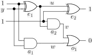
For example, the problem of diagnosing the full adder

circuit in Fig. 1 can be framed as a COP with variables

X = {u, v, w, y, a1, a2, e1, e2, o1}. Variables u to y describe boolean signals and have domain {0, 1}. Variables a1 to o1 describe the mode of each gate, which can either be G (good), S1 (shorted to input 1), S2 (shorted to input 2), or U (unknown failure). The COP has five constraints fa1, fa2, fe1, fe2, fo1, one for each gate in the circuit. Each constraint expresses that if the gate is G then it correctly performs its boolean function; and if it is S1 (S2) then it is broken such that its output equals its first (second) input; and if it is U then it is broken in an unknown way and no assumption is made about its behavior. The valuation structure captures the likelihood of being in a mode, and is ([0, 1],≥, ·, 1, 0) (with · being multiplication over the real numbers). We assume Or-gates have a .95

probability of being G, a .02 probability of being S1 (S2), and a .01 probability of being U; both And-gates and Xorgates have a .975 probability of being G, a .01 probability of being S1 (S2), and a .005 probability of being U. The value of the best solution then corresponds to the most likely fault in the circuit. For the example, α∗ is .018, corresponding to a stuck-at-first-input (S1) fault of Or-gate 1.

We introduce four more operators that we will use later to compare constraints and to turn them into hard constraints. The minimum operation, denoted min(f, g), returns the constraint whose valuation is the minimum of f(t) and g(t):

The sinking operation, denoted sink(f, g) returns the constraint that forbids t if f(t) ≥ g(t):

The lifting operation, denoted lift(f), turns a constraint into a hard constraint that allows t if f(t) < ⊤. Finally, the complement of a hard constraint f , denoted cmpl(f ), is the constraint whose valuation is ⊤ if f(t) = ⊥, and ⊥, otherwise.

3 Structure in Constraints

Our approach is based on exploiting independence properties of the constraint functions F, such that they can be represented more compactly (abstractly) than explicitly listing all assignments to X. In this section, we characterize these properties, which are often present in practical problems.

To start with, in many situations the valuation of a constraint will depend only on a subset of the variables. For instance, for the constraint fa1, its valuation depends only on a1, w, and y. Formally, the support of a constraint f is the subset of variables that it depends upon:

Definition 3 (Support) The support of a constraint f, denoted sup(f), is the variable set {xi ∈ X | ∃v1, v2 ∈ di s.t. (f ⊕ (xi ← v1)) ⇓X\{xi}̸= f ⊕ (xi ← v2)) ⇓X\{xi}}.

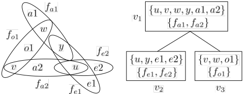
For the example, sup(fa1) = {a1,w, y}, sup(fa2) = {a2, u, v}, sup(fe1) = {e1, u, y}, sup(fe2) = {e2, u}, and sup(fo1) = {o1, v,w}. The support structure of a constraint problem can be abstractly represented through a hypergraph H that associates a node with each variable xi, and a hyperedge with the variables sup(fj) of each constraint fj. Fig. 3 shows the hypergraph for the example.

While the notion of support captures the independence of a function's value from variables outside the support, there can still exist independence within the support. For instance, in the constraint fo1, if o1 = S1 and v = 0, then the value is .02 regardless of the value of w; if o1 = U, then the value is .01 regardless of the values for w and y, etc. More generally, a property that we call weak support can be exploited: if the relationship between assignments and a function's value can be described more compactly than explicitly listing all the assignments to the support, then it is more efficient to solve problems on that symbolic level.

3.1 Symbolic Encoding using Decision Diagrams

In the following, we present a way to recognize support and

weak support of functions, namely through symbolic encoding in the form of decision diagrams. A decision diagram represents a function over boolean variables to a set of values. Binary decision diagrams (BDDs) [Bryant, 1986] represent functions with values 0 or 1; algebraic decision diagrams (ADDs) [Bahar et al., 1993] represent functions to any set of values. A decision diagram is a rooted, directed, acyclic graph, where each internal node corresponds to a boolean variable, and each leaf node corresponds to a value of the function. Internal nodes have two children n1, n2, and are recursively interpreted as the function f = if xi then f1 else f2, where xi is the boolean variable corresponding to the node, and f1 and f2 interpret the sub-diagrams with root nodes n1 and n2, respectively. The power of decision diagrams derives from their reduction rules and canonicity of representation. A decision diagram can be ordered by imposing a variable ordering x1 ≺ x2 ≺ . . . ≺ xn, such that for all paths from the root to the leaves, the sequence of variables encountered obeys the ordering. Ordered decision diagrams can be reduced by iteratively applying two graph reduction rules, which collapse assignments by sharing common prefixes and postfixes (to share a common postfix, the function value must be the same): the node deletion rule eliminates nodes from the diagram whose children are equal (n1 = n2), and the node sharing rule eliminates one of two nodes that are root nodes of isomorphic subdiagrams. A reduced, ordered decision diagram is a canonical representation of its function [Bryant, 1986] and contains only variables from the support of the function. It is easy to extend the technique to non-binary variables by mapping each non-binary variable xi to a block of ⌈log2 | Di |⌉ boolean variables that encode the domain values logarithmically. Figure 2 shows a reduced, ordered ADD representing the function fo1. Operations on functions, such as projection and combination, can be directly performed on this representation. The complexity of the operations depends on the size of the diagram (number of nodes and arcs), rather than on the number of possible assignments; due to the sharing of common substructures, the number of nodes and arcs can be orders of magnitude smaller than the number of possible assignments. While no compaction is achieved in the worst case, for certain types of constraints it can be shown that the size of the decision diagram grows only logarithmically with the number of assignments [Bryant, 1986].

4 Set-based Branch-and-Bound with Tree Decompositions

In this section, we describe how the independence properties of functions described in the previous section (support, weak support) can be exploited in the framework of branchand-bound search. We describe an algorithm that uses a tree decomposition of the hypergraph H to exploit the support of functions, and set-based search to exploit the weak support of functions. Thus, the algorithm benefits from compact representations of the functions, while memory explosion is avoided through depth-first search.

Figure 2: Constraint fo1 for the example in Fig. 1 and its

ADD, using two binary variables o11, o12 to encode o1, and

variable ordering o11 ≺o12 ≺v ≺w. Assignments and paths

with value 0 are not shown.

4.1 Tree Decomposition

Tree decomposition [Gottlob et al., 2000; Kask et al., 2003] is a way to exploit structural properties of H to decompose the original problem into independent subproblems ("clusters"):

Definition 4 (Tree Decomposition) A tree decomposition for a problem (X,D, F) is a triple (T, χ, λ), where T = (V,E) is a rooted tree, and χ, λ are labeling functions that associate with each node (cluster) vi ∈ V two sets χ(vi) ⊆ X and λ(vi) ⊆ F , such that

1. For each fj ∈ F, there exists exactly one vi such that fj ∈ λ(vi). For this vi, var(fj) ⊆ χ(vi) (covering condition);
2. For each xi ∈ X, the set {vj ∈ V | xi ∈ χ(vj)} of vertices labeled with xi induces a connected subtree of T (connectedness condition).

In addition, we demand that the constraints appear as close to the root of the tree as possible, that is,

1. If var(fj) ⊆ χ(vi) and var(fj) ̸⊆ χ(vk) with vk the parent of vi, then fj ∈ λ(vi).

Figure 3 shows a tree decomposition for the example. The separator of a node, denoted sep(vi), is the set of variables that vi shares with its parent node vj : sep(vi) = χ(vi)∩χ(vj). For convenience, we define sep(vroot) = ∅. Intuitively, sep(vi) is the set of variables that connects the subproblem rooted at vi with the rest of the problem:

Definition 5 (Subproblem) For a COP and a tree decomposition (T, χ, λ), the subproblem rooted at vi is the COP that consists of the constraints and variables in vi and any descendant vk of vi in T, with variables of interest sep(vi).

The subproblem rooted at vroot is identical to the problem of finding α∗ for the original COP. The benefit of a tree decomposition is that each subproblem needs to be solved only once (possibly involving re-using its solutions); the optimal solutions can be obtained from optimal solutions to the subproblems using dynamic programming. Thus, the complexity of constraint solving is reduced to being exponential in the size of the largest cluster only.

In order to exploit the decomposition during search, the variables must be assigned in an order that is compatible with the tree, namely by first assigning the variables in a cluster before assigning the variables in the rest of the subproblems rooted in the cluster. This is called a compatible order in [J´egou and Terrioux, 2003]. In [Terrioux and J´egou, 2003], J´egou and Terrioux present an algorithm called BTD (backtracking with tree decompositions) that exploits tree decompositions in branch-and-bound search. BTD assigns variables along a compatible order, beginning with the variables in χ(vroot). Inside a cluster vi, it proceeds like classical branchand-bound, taking into account only the constraints λ(vi) of this cluster. Once all variables in the cluster have been assigned, BTD considers its children (if there are any). Assume vj is a child of vi. BTD first checks if the restriction of the current assignment to the variables in sep(vj) has previously been computed as a solution to the subproblem rooted at vj . If so, the value of this solution (called a "good") is retrieved and combined with the value of the current assignment, thus preventing BTD from solving the same subproblem again (called a "forward jump" in the search). Otherwise, BTD solves the subproblem rooted at vj for the current assignment to sep(vj) and the current upper bound, and records the solution as a new good. Its value is combined with the value of the current assignment, and if the result is below the upper bound, BTD proceeds with the next child of vi.

4.2 Set-based Search

In the following, we generalize BTD from single assignments (and thus single bounds) to sets of assignment (and thus sets of bounds), in order to exploit symbolic representations of functions.

The method that we use to extend the search from single assignments to sets of assignments is to replace the step of assigning a value to a variable by the more general step of restricting a variable to a subset of its domain. This generalization is similar to domain splitting; however, whereas domain splitting might further split up the subsets at subsequent levels of the search tree, we consider the case where each variable occurs only once in each path of the search tree. That is, we assume that for each variable xi, a static, predefined partition of its domain into subsets is given:

Definition 6 (Domain Partition) A partition of a finite domain di is a set Pi of disjoint subsets of di whose union is di, that is, pj ∩pk = ∅ for pj , pk ∈ Pi, j ̸= k, and ⋃p∈Pi p = di.

There are two limiting cases: partitions consisting of singleton sets, that is, |Pi| = |di|, and partitions consisting of a single set containing all domain values, that is, |Pi| = 1. Again for notational convenience, we denote by xi ∈ p the restriction of a variable xi to the values in a partition element p, and a constraint over variable xi (its valuation is ⊥ if the value of xi is in p, and ⊤, otherwise).

The set-based algorithm proceeds by assigning partition elements p to variables xi, and computing lower bounds by combining the constraints all of whose variables have been assigned. Since a partition element can contain more than one domain value, the result is in general a function (set of assignments) rather than a single assignment. Thus, we need to generalize the basic test of the branch-and-bound algorithm - comparing a lower bound with an upper bound - to comparing two functions:

Proposition 1 Given a COP with variables of interest Z ⊆ X, let fu be a function with sup(fu ⊆ Z), and let fa be a set of assignments to Y ⊆ X (i.e., fa is a function with sup(fa ⊆ Y ). Then for an assignment t to Y , its extension t′ to all variables X can improve on fu (that is, (⊕mj=1 fj)(t) ⇓Z< fu(t)), if sink(fa ⇓Z, fu ⇓Z)(t) ̸= ⊤.

Hence, the sinking operation generalizes the comparison of a lower bound to an upper bound by "filtering out" assignments that cannot improve on a bounding function fu.

Algorithm 1 shows the pseudo-code for the resulting algorithm SBBTD (set-based branch-and-bound with tree decomposition). SBBTD is given a constraint fa (corresponding to a set of current assignments and their values), a cluster vi with a set of variables Yvi that remain to be assigned, and an upper bound function fu whose support is a subset of the variables sep(vi) (fu is a constant in the case where vi = vroot). SBBTD returns a constraint corresponding to the extension of assignments fa to solutions of the subproblem rooted at vi (again, the result is a constant in the case where vi = vroot). The valuation of this constraint is the value of best solution of the subproblem rooted at vi, or a value greater than or equal to fu(t), if this best value is greater than or equal to fu(t). SBBTD uses two functions Gvi , Rvi to record the goods (solutions to the subproblem rooted at vi) for each vi. Gvi is a soft constraint that contains the actual goods, while Rvi is a hard constraint that contains the information whether an assignment has been recorded as a good or not (the use of two functions is necessary because a good can have any value in E, thus function Gvi alone cannot give sufficient information whether the good has been stored or not). That is, an assignment t is recorded as a good for the separator if Rvi (t) = ⊤, and not recorded if Rvi (t) = ⊥; in case the good is recorded, its value is Gvi (t). Initially, Rvi = Gvi = ⊥.

SBBTD starts by filtering out the assignments whose value exceeds the bounding function (line 1). Inside a cluster (lines 19-28), SBBTD operates like branch-and-bound, except that it restricts variables to subsets of their domains (partition elements) instead of single values. Once all variables in the cluster have been assigned, SBBTD turns to its children (lines 3-17). SBBTD chooses a child vj and first computes the subset of assignments f ′a of fa that are not previously recorded as goods of sep(vj) (line 7). If there are any assignments

SBBTD(fa, vi, Yvi , fu) 1: fa ← sink(fa, fu) 2: if Yvi = ∅ then 3: F ← children(vi) 4: while F ̸= ∅ and fa ̸= ⊤ do 5: choose vj ∈ F 6: F ←F \ vj 7: f ′a ← Rvj ⊕ fa 8: if f ′a ̸= ⊤ then 9: ha ← lift(f ′a ) ⇓sep(vj ) 10: ea ← SBBTD(ha, vj ,χ(vj )\sep(vj ),fu ⇓sep(vj )) 11: Gvj ← Gvj ⊕ (ea ⊕ ha) 12: Rvj ←Rvj ⊕ compl(ha) 13: end if 14: fa ← fa ⊕ Gvj 15: fa ← sink(fa, fu) 16: end while 17: return fa ⇓sep(vi) 18: else 19: choose xi ∈ Yvi 20: S ←Pi 21: I ← {f ∈λ(vi): xi ∈ sup(f), sup(f)⊆sup(fa)∪xi} 22: while S ̸= ∅ and fa ̸= ⊤ do 23: choose p ∈ S 24: S ←S \ p 25: f ′a ← fa ⊕ (xi ∈ p) ⊕f∈I f 26: fu ← min(fu, SBBTD(f ′a , vi, Yvi \ {xi}, fu)) 27: end while 28: return fu 29: end if

not recorded as goods, SBBTD solves the subproblem rooted at vj for these assignments (line 10), and records the solutions as new goods (lines 11 and 12). It updates the values of the current assignments fa (lower bounds) (line 14), and compares it with the current upper bounds (line 15). It continues with the next child (if any) or returns the solutions to the subproblem. The initial call to the algorithm is SBBTD(⊥, vroot, χ(vroot), ⊤).

Since the formulation of the algorithm is independent of how the domain partitions are defined, Fig. 1 actually defines a spectrum of algorithms that is parameterized by the domain partitions Pi for each variable. The limiting cases of the spectrum are |Pi| = |di| and |Pi| = 1, corresponding to finest and coarsest granularity of the domain partitions, respectively. In the first case, the set of assignments fa actually consists of a single assignment with value smaller than ⊤, and thus Alg. 1 becomes identical to branch-and-bound on tree decompositions (BTD). In the second case, the restrictions xi ∈ p yield constraints identical to ⊥, and thus the search tree degenerates to a list. Hence, in this case the algorithm is backtrackfree and becomes identical to dynamic programming on the tree (called cluster-tree elimination (CTE) in [Kask et al., 2003]). For the cases in between, that is, 1 < |Pi| < |di|, hybrids of search and dynamic programming are obtained.

Theorem 1 For a COP (X,D, F) with a tree decomposition (T, χ, λ) and any domain partitions P1, P2, . . . , Pn for variables x1, x2, . . . , xn, the algorithm SBBTD is sound and complete, that is, SBBTD(⊥, vroot, χ(vroot), ⊤) = α∗ .

For instance, consider the full adder example with the domain partitions Pu, Pv = {{0},{1}}, Pw, Py = {{0,1}}, and Pa1, . . . , Po1 = {{G},{S1,S2},{U}}. That is, the search simultaneously explores the values {0,1} for w and y and the values {S1,S2} for the mode variables. SBBTD starts by assigning the variables {u, v,w, y, a1, a2} in the cluster v1, which gives two assignments, 〈u, v,w, y, a1, a2〉 = 〈0, 0, 0, 0,G,G〉 and 〈0, 0, 1, 1,G,G〉, both with value .95. SBBTD next considers a child of v1, for instance, v2. Since there are no goods recorded for this cluster so far, the solutions are computed for this subproblem for the assignments 〈u, y〉 = 〈0, 0〉 and 〈0, 1〉. The value of these solutions are .0097 (corresponding to a S2 failure of Xor-gate 1) and .95, respectively. These solutions are recorded and combined with the two assignments, which now have the values .0092 and .90, respectively. Next, the solutions for the subproblem v3 are computed simultaneously for the assignments 〈v,w〉 = 〈0, 1〉 and 〈0, 1〉. The values are .95 and .01 (corresponding to a S1 failure of the Or-gate), respectively. After combining these solutions with the two assignments in v1, their value becomes .0088 and .018, respectively. Since there are no children left, SBBTD updates the bound for the best solution found to .018. This bound prunes all subsequent assignments to variables in v1 except 〈u, v,w, y, a1, a2〉 = 〈1, 1, 0, 0, G, G〉 and 〈1, 1, 1, 1, G, G〉. Since the assignments 〈u, y〉 = 〈1, 0〉 and 〈1, 1〉 for the subproblem v2 lead to values worse than the bound, .018 is returned as optimal solution.

In comparison, observe that BTD (obtained as a specialization of SBBTD for the case |Pi| = |di|) suffers from the problem that it would explicitly iterate through all possible combinations of values for w and y until encountering the best assignment (which is obtained for 〈w, y〉 = 〈1, 1〉); in contrast, SBBTD handles those combinations implicitly. Dynamic programming (obtained as a specialization of SBBTD for |Pi| = 1) suffers from the problem that it would consider more assignments than necessary (for example, it would compute the value for assignments involving 〈a1, a2〉 = 〈U,U〉, which is very low because it corresponds to a double fault).

4.3 Trade-off between Search and Symbolic Inference

SBBTD unifies search with good recording (BTD) and dynamic programming (CTE). In fact, the goods that the BTD algorithm computes can be understood as partial construction of the messages sent between clusters by the dynamic programming algorithm CTE [Kask et al., 2003]. Thus, the two limiting cases can be understood as lazy and eager forms of dynamic programming, respectively: BTD computes solutions to subproblems only as far as required to compute the optimal solution, whereas CTE computes them completely.

It has been previously shown [J´egou and Terrioux, 2003] that BTD (i.e., lazy dynamic programming) outperforms CTE (i.e., eager dynamic programming). This is because search on single assignments exploits the upper bounds as rigorously as possible, and therefore the least number of assignments will be explored. However, this argument is based on counting assignments and holds only if assignments are represented explicitly. The picture changes when using techniques such as ADDs that can manipulate sets of assignments implicitly. Hence, a tension is created between making the partition elements in SBBTD smaller or larger: in the former case, the advantage is that as few assignments are explored as possible, but the disadvantage is that less possibilities exist for exploiting commonalities between assignments. In the latter case, the disadvantage is that more assignments might be explored, but the advantage is that assignments can be abstracted into a more compact description and handled implicitly. Thus in many practical cases, the optimal granularity will lie in an intermediate point (1 ≤ |Pi| < |di|) along the spectrum; SBBTD allows us to adapt to this trade-off.

5 Implementation and Experiments

We implemented SBBTD using the CUDD (Colorado University Decision Diagram) package [Somenzi, 2004], which provides a library of routines for manipulating ADDs.

We evaluated the performance of this prototype on random, binary Max-CSP problems. Max-CSP is a constraint optimization problem where the tuples of a constraint have cost 0 if the tuple is allowed, and cost 1 if the tuple is not allowed; the optimal solution corresponds to an assignment that violates a minimum number of constraints. For each instance, the support of the constraints was determined in order to derive the hypergraph (a graph in this case). Then, a tree decomposition of the hypergraph was computed using the min-fill heuristics. We choose random domain partitions, whose granularity we varied by setting a certain percentage P of (random) variables to the partition |Pi| = 1, and the other variables to the partition |Pi| = |di|. We ran the experiments on a Pentium 4 Windows PC with 1 GB of RAM; due space restrictions we give only summarized results here.

Consistent with results in [J´egou and Terrioux, 2003], we found the number of assignments explored for P=0% (BTD) to be in most cases several times smaller than the number of assignments explored for P=100% (dynamic programming). E.g., in an example class with N=40 variables, C=80 constraints, domain size K=4 and tightness T=9, the mean number of goods recorded for P=0% was 50,00 to 100,000, whereas for P=100% it was 250,000 to 1,000,000. However, the ADD representation of constraints typically achieved a compaction of around one to two orders of magnitude (consistent with observations in [Hoey et al., 1999]). Therefore, and also because larger partition elements reduce the number of recursive calls, SBBTD ran faster for larger values of P in almost all cases. E.g., for N=40, K=4, C=80 and T=9, the mean runtime for P=0% was around 100 sec, but around 0.5 to 1 sec for P=100%. Given that for P=100% the computation required up to one order of magnitude more memory than P=0%, selecting an intermediate granularity (0% < P < 100%) allowed significant runtime improvements over BTD within still acceptable memory bounds. We are currently working on structured examples (like in [J´egou and Terrioux, 2003]) and real-world examples.

6 Conclusion

We presented an algorithm for solving soft constraint problems by generalizing branch-and-bound to search on sets of assignments and perform inference (dynamic programming) within those sets of assignments. This hybrid approach can exploit regularities in the constraints, while it can avoid memory explosion by controlling the size of the sets. In contrast to work in [Hoey et al., 1999; Jensen et al., 2002], our approach is more general in that it addresses valued constraint satisfaction problems [Schiex et al., 1995], and incorporates a decomposition of the problem into several subproblems. Future work includes ways to automatically determine domain partitions (appropriate points in the spectrum), and augmenting the algorithm with symbolic versions of constraint propagation techniques [Cooper and Schiex, 2004] in order to further improve the bounds.