The COMPSET Algorithm for Subset Selection

1 Introduction

The subset selection problem (SSP) is simply defined: Given a set of elements E = {e1, e2, . . . , en} and a utility function U : 2E ↦→ R, find a subset S ⊆ E such that U(S) is optimal. Many real-life problems are SSPs, or can be formulated as such. Classic examples include SAT, max clique, independent set, vertex cover, knapsack, set covering, set partitioning, feature subset selection (classification) and instance selection (for nearest-neighbor classifiers) to name a few.

Since the search space is exponential in the size of E, finding an optimal subset without relaxing assumptions is intractable. Problems associated with subset selection are typically NP-hard or NP-complete. Local search algorithms are among the common methods for solving hard combinatorial optimization problems such as subset selection. Hill climbing, simulated annealing [Kirkpatrick et al., 1983] and tabu search [Glover and Laguna, 1993] have all been proven to provide good solutions in a variety of domains. The general technique of random restarts is applicable to all of them, yielding anytime behavior as well as the PAC property (probability to find the optimal solution converges to 1 as the running time approaches infinity).

The problem with these local search algorithms is, however, that they are too general. The only heuristic they have about the domain is in a form of a black-box, the utility function which they try to optimize. It is therefore common to have modifications to these algorithms that trade being general for additional domain-specific knowledge. The SAT domain is full of such variants [Gent and Walsh, 1993; Hoos and St¨ utzle, 2005] but they are common in other domains as well [Khuri and B¨ ack, 1994; Evans, 1998].

In this paper we present a general modification to known local search algorithms which improve their performance on SSPs. The idea behind it is to exploit attributes that are specific to search spaces of subset selection. Knowing that it is a subset search space allows us to infer which moves were likely to be wrong. By reversing these moves and trying again, we start from a new context, and the probability to repeat the mistake is reduced. In experiments performed on complex SAT, max clique, 0/1 multidimensional knapsack and vertex cover problems, the new method has shown to significantly improve the underlying search algorithm.

2 The COMPSET Algorithm

Subset selection can be expressed as a search in a graph. Each node (state) in the graph represents a unique subset. Edges correspond to adding or removing an element from the subset, thus there are n = |E| edges to every node. The following figure shows the search graph for 3 elements.

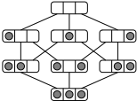
A state S can be represented by a bit vector where bit S[i] is 1 iff ei ∈ S. Moving to a neighboring state in the graph is equivalent to flipping one bit.

Each state is associated with a utility value, which is the value of U on the subset it represents. Local search algorithms typically start from a random state and make successive improvements to it by moving to neighboring states. They vary from each other mainly in their definition of neighborhood, and their selection method.

Using this representation, all local search algorithms are also applicable to subset selection. However, being general, they overlook the specific characteristics of subset selection. COMPSET guides a given local search algorithm using knowledge specific to subset selection.

2.1 Characteristics of Subset Selection

In a selection problem of n elements, there are n operators: F = {f1, f2, . . . , fn} where fi is the operator of toggling the membership of element i in a set (if it was in the set remove it , or add it if it was out). Applying fi is equivalent to flipping the ith bit in the bit vector representation. Throughout the following discussion we assume a single optimal subset (solution) which we donate S∗ .

We make the following observations about subset search:

Observation 1. Let S′ be an arbitrary state (subset). From any state S, there exists a subset of the operators, σ(S, S′ ) ⊆ F, that when applied to S results in S′ .

Proof. Since S′ , as S, is an n bits long vector, there are at most n bits of S′ that do not agree with S and need to be flipped using an operator.

Observation 2. Let S be the complementary state of S i.e., the state derived from S by flipping all its bits. The subset of operators σ(S, S∗ ) leading from S to the solution S∗ , is the complementary subset of σ(S, S∗ ) in F. That is, σ(S, S∗ ) ∪ σ(S, S∗ ) = F and σ(S, S∗ ) ∩ σ(S, S∗ ) = ∅.

Proof. We need to show, that for every fi∈F either fi ∈ σ(S, S∗ ) or fi ∈ σ(S, S∗ ). If S[i] = S∗ [i] then fi /∈ σ(S, S∗ ) (it does not need to be flipped). Moreover, if S[i] = S∗ [i] , then necessarily S[i] ̸= S∗ [i] , since in S all bits are flipped. Thus, fi /∈ σ(S, S∗ ) → fi ∈ σ(S, S∗ ). The same goes for the other possible case, in which S[i] = S∗ [i] .

The inherent problem in finding σ(S, S∗ ) using local search, is that operators are applied successively and their effect is not necessarily of monotonic improvement due to interdependencies between elements. Such non-monotonic behavior of U confuses local search algorithms and often makes them trapped in local optima. In such a case, there are two options: either the search is progressing on the correct path to the solution (but the algorithm does not see a way of continuing), or it is off the correct path altogether. It would be beneficial to distinguish between these two scenarios.

Consider two independent hill climbing runs, one from S and one from S. Given that the optimal solution is not found, the two runs have stopped in local optima, LS and LS respectively. We consider the subsets of operators leading from S to LS and from S to LS . By observation 2, it is not possible that an operator fi appears in both operator subsets if they are both on the path to S∗ . If we do observe the same operator in both, it is a clear sign that one of them is wrong. This is the idea behind COMPSET, which is described next.

2.2 Description of the COMPSET Algorithm

Interdependencies between elements are distracting when searching for good solutions. Had all elements been independent, a simple linear search, which adds element after element as long as the utility value improves, would suffice. Local optima are an example where such interdependency brings the search to a full stop. It is likely that by applying the operators in a different order, or eliminating some, the local optimum would have been avoided. COMPSET uses the above observations to try and identify wrong invocations of operators. It then cancels them (reverses their effect) and resumes the run towards another local optimum or, hopefully, the solution.

Procedure COMPSET(S, LOCALSEARCHALG)

S1 ← S ; S2 ← S ; agree ← false loop until agree LS ← LOCALSEARCHALG(S1) LS ← LOCALSEARCHALG(S2) C ← σ(S, LS) ∩ σ(S, LS ) if C is empty then agree ← true else S1 ←C(LS) // apply all operators in C on LS S2 ← C(LS ) return the better between LS and LS

end

Given a start state S, COMPSET initiates two runs of the given local search algorithm, one from S and one from its complementary S. Once two local optima are achieved, the series of operators that has led to each one is examined. Every operator that appears in both series must be wrong in one of them. We do not know which of the runs went wrong, so we reverse the effect of such operators in both local optima. Once all obviously wrong operators are undone, the local search is continued. The process repeats upon encountering the next pair of local optima. When no conflicting operators exist, and the optimal solution was not found, COMPSET ends and returns the better of the two local optima in hand.

The rational behind COMPSET is illustrated here:

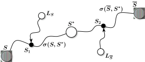
The solution S∗ is reachable by applying all operators from σ(S, S∗ ) to S (in any order), and by applying all operators from σ(S, S∗ ) to S. The underlying search algorithm from S is in a correct path if it is using only operators from σ(S, S∗ ).

However, a search can easily divert from this path, and it is often necessary for its overall convergence to the solution. Diversion occurs if an operator from σ(S, S∗ ) is applied to S, or an operator from σ(S, S∗ ) is applied S. The problem is, that since we do not know σ(S, S∗ ) or σ(S, S∗ ), it is difficult to detect such diversions. However, what we do know, is that the solution S∗ conforms to σ(S, S∗ ) ∩ σ(S, S∗ ) = ∅. We can use this fact to try and identify diversions.

Once stopped in local optima LS from S and LS from S, we check σ(S,LS) ∩ σ(S,LS ). If the intersection is not empty then by definition either LS or LS are off the path. Note, that if the intersection is empty, the local optima might still be off path, because either σ(S,LS) uses an operator from σ(S, S∗ ), or σ(S, LS ) uses an operator from σ(S, S∗ ). However, σ(S,LS) ∩ σ(S,LS ) ̸= ∅ means that for sure at least one of the local optima is off path.

In general it is possible that the search algorithm would continue applying operators and finally return to the path, but being in a local optimummeans that it has essentially "given up". Elimination of all conflicting operators from both sides brings us to S1 and S2, LS → S1 and LS → S2. Since all common operators were eliminated, σ(S, S1) ∩ σ(S, S2) = ∅ and thus S1 and S2 are on a possibly correct path. It is still possible that σ(S, S1) contains operators from σ(S, S∗ ) or that σ(S, S2) contains operators from σ(S, S∗ ) thus still being an obstacle for reaching the solution.

An important point to notice, is that S1 and S2 are not necessarily states that the algorithm has visited before. Groups of operators are simultaneously eliminated, an operation which interdependencies would prohibit had the operators were successively eliminated. COMPSET effectively switches to another context which is mostly correct, in which the eliminated operators can be tried again.

3 Empirical Evaluation

The following algorithms were considered:

• Stochastic Hill Climbing (SHC) - starts from a random subset, iteratively picks a neighboring subset (differs in exactly one element) in random and moves there if it has a better or equal utility value. The simplicity of SHC often misleads; several works [Mitchell et al., 1994; Baluja, 1995] showed that SHC does not fall from the complex GA mechanism. In the SAT domain such stochastic local search (SLS) methods have been shown to be comparable with state-of-the-art domain-specific algorithms [Hoos and St¨ utzle, 2005].
• Tabu Search (TS) [Glover and Laguna, 1993] - examines the neighborhood of the current state for the best replacement. It moves to the chosen state even if it does not improve the current state, which might result in cycles. To avoid cycles, TS introduces the notion of a tabu list that stores the last t (tabu tenure) operators used. TS is prevented from using operators from the tabu list when it generates the neighborhood to be examined, unless certain conditions called aspiration criteria are met. In this paper we use a common aspiration criterion that allows operators which lead to better state than the best obtained so far.
• Simulated Annealing (SA) [Kirkpatrick et al., 1983] - begins at high temperature which enables it to move to arbitrary neighboring states, including those which are worse than the current one. As the temperature declines, the search is less likely to choose a non-improving state, until it settles in a state which is a local minimum from which it cannot escape in low temperatures.

To test the effectiveness of COMPSET we have applied it to SHC and TS. COMPSET is not applicable to SA since SA begins with a high temperature at which it randomly moves far from the initial state. The concept of COMPSET is to set new start points for the underlying algorithm and by randomly moving away from them SA defeats its purpose.

The algorithms were tested in the following domains:

• Propositional Satisfiability (SAT) - the problem of finding a truth assignment that satisfies a given boolean formula rep-

resented by a conjunction of clauses (CNF) C1 ∧ . . . ∧ Cm. SAT is a classic SSP since we look for a subset of variables that when assigned a true value, makes the entire formula true. The utility function is the number of unsatisfied clauses when assigning true to all variables in S:

The global minimum for U is 0, for satisfied formulas. A search algorithm using this utility function will attempt to maximize the number of satisfied clauses, which is a generalization of SAT called MAX-SAT. Problem instances for SAT were obtained from the SATLIB [Hoos and St¨ utzle, 2000] repository of random 3-SAT. We use problems from the solubility phase transition region 1 [Cheeseman et al., 1991].

• Max Clique - another classic SSP, where the goal is to find the maximum subset of vertices that forms a clique in a graph. Given a graph G = (V, E) and a subset S ⊆ V , we define the following utility function:

A clique should be maximized but our implementation always minimizes U, therefore we use |V | - |S|. Incomplete solutions are penalized by the number of additional edges they require for being a clique (|S| · (|S| - 1) - |ES|), plus a fixed value |V | that is used to separate them from the legal solutions. By striving to minimize U, the search algorithm finds feasible solutions first, and then continues by minimizing their size. The global minimum of U corresponds to the maximum clique. Problem instances were obtained from the DIMACS [1993] benchmark for maximum clique.

• 0/1 Multidimensional Knapsack (MKP) - the problem of filling m knapsacks with n objects. Each object is either placed in all m knapsacks, or in none of them (hence "0/1"). The knapsacks have capacities of c1, c2, . . . , cm. Each object is associated with a profit pi and m different weights, one for each knapsack. Object i weighs wij when put into knapsack j. The goal is to find a subset of objects yielding the maximum profit without overfilling any of the knapsacks. Knapsack j is overfilled in state S iff ∑ni=1 S[i] · wij > cj.

Let k be the number of overfilled knapsacks. We define:

The utility of feasible subsets is simply their profit (with minus sign for minimization purposes). Infeasible solutions are penalized for each knapsack they overfill. Problem instances for MKP were obtained from the OR-library [Beasley, 1997].

• Vertex Cover - the goal is to find the smallest subset of vertices in a graph that covers all edges. Given a graph G = (V, E), we define:

1 Random 3-SAT problem with 4.26 clauses per variable that are the hardest to solve using local search.

For legal vertex covers, U takes values less than or equal to |V |. Incomplete solutions are penalized by the number of edges they do not cover, plus a fixed value |V | that is used to separate them from the legal solutions. The global minimum of U corresponds to the optimal vertex cover.

The complementary graphs of the instances from the original DIMACS benchmark were taken, so that the known maximum clique sizes could be translated to corresponding minimum vertex covers 2 .

3.1 Experimental Methodology

We have tested five algorithms: SHC, TS, SA (with T = 100, α = 0.95), COMPSET over SHC and COMPSET over TS. TS was used with t = 5 for all domains other than SAT, and t = 9 for SAT. Each run was limited to 107 U evaluations.

All algorithms use random restart to escape from local optima when they have still not exhausted their evaluations quota. They use random restart also when there is no improvement over the last k steps. We use k = 10 for domains other than SAT, and k = 20 for SAT. SAT is characterized by wide and frequent plateaus [Frank et al., 1997] therefore we chose higher values of t and k for it.

100 runs of each algorithm were performed on each problem in the test sets. Each run started from a random state, that was common to all algorithms. We measured the number of U evaluations needed to obtain the optimal solution in each run, as well as the time taken.

3.2 Results

The results are summarized in Tables 1, 2, 3 and 4. For brevity, we did not include the timing information in these tables. The considered algorithms do not introduce a significant overhead, so the execution time is a linear function of the number of U evaluations. The tables show the characteristics of the problem instance, followed by the number of successful runs (columns titled #ok) and the average number of U evaluations for each algorithm. A successful run is a run in which the algorithm has found the optimal solution within the limit. We tested the statistical significance of the improvement introduced by COMPSET using the Wilcoxon matched-pairs signed-ranks test with the extension by Etzioni and Etzioni [1994] to cope with censored data 3 . A "+" sign in the sg. column between SHC and COMPSET/SHC indicates that COMPSET improved SHC with p < 0.05. A "-" sign indicates that SHC performed better with p < 0.05. A "?" sign indicates that the difference is not significant. Whenever it is not possible to draw definitive conclusions since there is too much censored data, n/a appears. The same holds for the sg. column between TS and COMPSET/TS.

The superiority of COMPSET over the other algorithms is striking, both in the number of evaluations, and the number and difficulty of instances solved. In the SAT domain, the best performing algorithms are COMPSET/TS and COMPSET/SHC. The average success ratio of COMPSET/TS is 85% and of COMPSET/SHC is 76%. For comparison, the success ratios for SA, TS and SHC are 37%, 23% and 28% respectively. The speedup factor gained by using COMPSET is as large as 462 for SHC (instance uf50-011) and as large as 156 for TS (instance uf75-013). Note that these are lower bounds since SHC and TS were terminated because of resource limit for some of the runs.

2 Note that while it is possible to take the complementary graph, solve the Max Clique problem, and then translate back to Vertex Cover, none of the algorithms in this paper has done so.

3 The information about runs in which the solution was not found within the given bound is called truncated or censored.

The best performing algorithms in the Max Clique domain are COMPSET/SHC and SHC with average success ratios of 94% and 80% respectively. The speed up factor of COMPSET/SHC over SHC is as large as 14 (instnace sanr200 0.7).

In the Knapsack domain, the best performing algorithm is COMPSET/SHC with an average success ratio of 89%. For comparison, the success ratios for TS, SA, COMPSET/SHC and SHC are 50%, 25%, 19% and 17% respectively. The speedup factor gained by using COMPSET is as large as 127 for TS (instance WEISH07) and as large as 3.8 for SHC (instance WEISH04).

The best performing algorithms in the Vertex Cover domain are COMPSET/SHC and SHC with average success ratios of 94% and 77% respectively. SA is relatively close with 71% but TS is far behind with 23%, improved by COMPSET to 28%. The speedup factor gained by using COMPSET is as large as 310 for TS (instance hamming6-2) and as large as 10 for SHC (instance sanr200 0.7).

Another interesting statistics is the number of random restarts required by the underlying search algorithm and COMPSET, as well as the number of operator eliminations performed by COMPSET and how many operators they spanned. We have collected this data throughout 100 runs on the p hat1000-1 vertex cover problem, a graph of 1000 vertices. SHC required 517.37 random restarts on average (in each run), while COMPSET required only 3.13. COMPSET has performed 20.52 operator eliminations, reversing the effect of 2.97 operators each time.

4 Conclusions and FutureWork

In this paper, we have provided useful insights into the domain of subset selection. We have realized that using local search, paths from complementary subsets to the solution must be distinct in terms of the operators used. This has led us to conclude that if the paths contain common operators, it may serve as an indication of a mistake. To test our conjecture, we introduced COMPSET, a new guiding policy for local search algorithms in the context of SSP. The results show a significant improvement over both TS and SHC by up to two orders of magnitudes.

We currently in the process of running COMPSET on other subset selection domains, progressing towards a better understanding of its behavior. One interesting direction is to research for ways to incorporate knowledge of the entire search paths, instead of only the local minima at their end. In addition, it is beneficial to find out how characteristics of a specific problem affect its performance. Overall, the general idea of incorporating such SSP specific insights seems to be a promising lead to better subset selection algorithms.