
Efficient Stochastic Local Search for MPE Solving
Proceedings of the Nineteenth International Joint Conference on Artificial Intelligence. Pages 169-173.
© 2005 International Joint Conferences on Artificial Intelligence
Abstract
Finding most probable explanations (MPEs) in graphical models, such as Bayesian belief networks, is a fundamental problem in reasoning under uncertainty, and much effort has been spent on developing effective algorithms for this N P-hard problem. Stochastic local search (SLS) approaches to MPE solving have previously been explored, but were found to be not competitive with state-of-theart branch & bound methods. In this work, we identify the shortcomings of earlier SLS algorithms for the MPE problem and demonstrate how these can be overcome, leading to an SLS algorithm that substantially improves the state-of-the-art in solving hard networks with many variables, large domain sizes, high degree, and, most importantly, networks with high induced width.
- [Boykov et al., 2001] Y. Boykov, O. Veksler, and R. Zabih. Fast approximate energy minimization via graph cuts. PAMI, 23(11), 2001.
- [Cowell et al., 1999] R. G. Cowell, A. P. Dawid, S. L. Lau- ritzen, and D. J. Spiegelhalter. Probabilistic Networks and Expert Systems. Statistics for Engineering and Information Science. Springer, 1999.
- [Dechter and Rish, 2003] R. Dechter and I. Rish. Mini- buckets: A general scheme for bounded inference. J. of the ACM, 50(2):107-153, 2003.
- [Dechter, 1999] R. Dechter. Bucket elimination: A unifying framework for reasoning. AIJ, 113(1-2):41-85, 1999.
- [Hoos and Stützle, 2004] H. H. Hoos and T. Stützle. Stochastic Local Search -Foundations & Applications. Morgan Kaufmann, SF, CA, USA, 2004.
- [Hutter, 2004] F. Hutter. Stochastic local search for solving the most probable explanation problem in Bayesian net- works. Master's thesis, Darmstadt University of Technol- ogy, Darmstadt, Germany, September 2004.
- [Jaakkola and Jordan, 1999] T. S. Jaakkola and M. I. Jordan. Variational probabilistic inference and the QMR-DT net- work. JAIR, 10:291-322, 1999.
- [Kask and Dechter, 1999] K. Kask and R. Dechter. Stochas- tic local search for Bayesian networks. In Proc. of AISTATS-99, January 1999.
- [Marinescu and Dechter, 2004] R. Marinescu and R. Dechter. AND/OR tree search for constraint opti- mization. In Soft'04 workshop at CP'2004, 2004.
- [Marinescu et al., 2003] R. Marinescu, K. Kask, and R. Dechter. Systematic vs. non-systematic algorithms for solving the MPE task. In Proc. of UAI-03, 2003.
- [Mills and Tsang, 2000] P. Mills and E. P. K. Tsang. Guided local search for solving SAT and weighted MAX-SAT problems. In SAT2000, pages 89-106. IOS Press, Ams- terdam, The Netherlands, 2000.
- J. D. Park. Using weighted MAX-SAT engines to solve MPE. In Proc. of AAAI-02, pages 682-687, 2002.
- [Pearl, 1988] J. Pearl. Probabilistic Reasoning in Intelligent Systems: Networks of Plausible Inference. Morgan Kauf- mann, SF, CA, USA, 1988.
- [Rish et al., 2002] I.
- Rish, M. Brodie, and S. Ma. Accu- racy vs. efficiency trade-offs in probabilistic diagnosis. In Proc. of AAAI-02, pages 560-566, 2002.
- [Tappen and Freeman, 2003] M. F. Tappen and W. T. Free- man. Comparison of graph cuts with belief propagation for stereo, using identical MRF parameters. In Proc. of ICCV-03, volume 2, pages 900 -906, 2003.
- [Voudouris and Tsang, 1999] C. Voudouris and E. P. K. Tsang. Guided Local Search and its application to the trav- elling salesman problem. EJOR, 113(2):469-499, 1999.
- [Yanover and Weiss, 2003] C. Yanover and Y. Weiss. Ap- proximate inference and protein-folding. In Proc. of NIPS- 02, pages 1457-1464, 2003.
- [Yedidia et al., 2002] J.S Yedidia, W.T. Freeman, and Y. Weiss. Understanding belief propagation and its gen- eralizations. Technical report, Mitsubishi Electrical Re- search Laboratories Inc., TR-2001-22, 2002.
References were extracted automatically from the PDF and may contain errors.
Full text extracted automatically from the PDF; figures, tables and equations may differ. The PDF is the version of record.
1 Introduction
Since Pearl's classic text [Pearl, 1988], graphical models such as Bayesian networks have become the prime representation for uncertainty in AI. This paper deals with the problem of finding the Most Probable Explanation (MPE) for some evidence when reasoning under uncertainty. More specifically, in the light of uncertain knowledge represented as a probabilistic graphical model, this problem is cast as finding the most probable instantiation of all the model's variables V given the observed values e for a subset E ⊆ V.
The MPE problem in graphical models has applications in different fields, such as medical diagnosis [Jaakkola and Jordan, 1999], fault diagnosis [Rish et al., 2002], computer vision [Tappen and Freeman, 2003], and prediction of sidechains in protein folding [Yanover and Weiss, 2003], to name just a few. Consequently, many algorithms have been suggested to solve this problem, but since it is NP-hard, many hard problem instances still cannot be solved efficiently. The available algorithms for MPE solving include exact methods like variable elimination (VE) [Dechter, 1999], junction tree (JT) [Cowell et al., 1999] and conditioning techniques [Pearl, 1988], but also systematic search algorithms, such as branch & bound (B&B), guided by a Mini-Buckets (MB) heuristic [Dechter and Rish, 2003]. Since in practice many applications require efficient online algorithms for networks of high induced width, there is also much research
Thomas St ¨ utzle
Computer Science Dept. Darmstadt Univ. of Technology Darmstadt, Germany stuetzle@informatik.tu-darmstadt.de
in approximate MPE algorithms, reaching from loopy belief propagation (BP) [Pearl, 1988] and generalized BP [Yedidia et al., 2002] to stochastic local search (SLS) algorithms [Kask and Dechter, 1999; Park, 2002] and specialized algorithms, such as graph cuts for certain pairwise Markov Random Fields (MRFs) that, for example, occur in computer vision [Boykov et al., 2001].
B&B approaches have recently been shown to be stateof-the-art methods in MPE solving, and it has been claimed that for MPE, B&B algorithms clearly outperform GLS, the best performing SLS algorithm known so far, in terms of the ability to find high-quality solutions quickly [Marinescu et al., 2003]. This is in stark contrast to results for numerous other combinatorial optimisation problems, such as weighted MAX-SAT, where SLS algorithms clearly define the state-ofthe-art (see, e.g., [Hoos and St¨ utzle, 2004]).
In this work, we analyse the shortcomings of previous SLS algorithms for MPE and demonstrate that these weaknesses can be overcome based on the careful consideration of important issues, such as the time complexity of individual search steps, search stagnation and thorough parameter tuning. In particular, we introduce improvements to Park's GLS algorithm [Park, 2002] that overcome its inferior scaling behaviour with network and domain size. Our new algorithm, GLS+, clearly outperforms current state-of-the-art MPE algorithms on various types of networks, especially for hard networks with high induced width, and hence establishes stochastic local search as a highly attractive and competitive approach to MPE solving.
The remainder of this paper is structured as follows. We first introduce some basic concepts and notation in Section 2; next, in Section 3, we describe GLS and GLS+ and present some computational results illustrating the improvement of GLS+ over GLS. In Section 4 we present empirical results that establish GLS+ as a new state-of-the-art algorithm for finding MPEs. We close with some conclusions and a brief outlook on future work in Section 5.
2 Preliminaries
A discrete Bayesian belief network (or Bayes net) B is a quadruple 〈V,D, G,Φ〉, where V is an ordered set of random variables, D is an ordered set of finite domains DVi for each Vi ∈ V, G = (V, E) is a directed acyclic graph (DAG), and Φ is an ordered set of CPTs φV = P(V |pa(V )), specifying the conditional probability distribution of each V ∈ V
given its parents pa(V ) in G. Semantically, a Bayes net specifies a joint probability distribution φ over its variables V in factored form: φ = P (V) = ∏V ∈V φV .
Given a Bayes net B = 〈V, D, G, Φ〉 and a set of evidence variables E = e, the Most Probable Explanation (MPE) problem is to find an instantiation V = v with maximal probability p(v) := ∏φ∈Φ φ[V = v] over all variable instantiations v consistent with evidence e. While all networks in our experimental analysis are Bayes nets, our algorithms are equally applicable to other graphical models, such as MRFs or general factor graphs.
CPTs are a special case of potentials, which are functions that have non-negative entries for any assignment of their variables. One well-known method for solving MPE in general networks is variable elimination (VE) (see, e.g., [Dechter, 1999]); it iteratively eliminates variables V by multiplying all potentials that are defined over V and then maximizing V out of the product thus obtained. Once all variables are eliminated, the best assignment can be recovered in linear time. Mini-Buckets with i-bound ib (MB(ib)) [Dechter and Rish, 2003] approximates VE by splitting each product into smaller products with at most ib variables; MB-w(s) is a new variant of MB that instead limits the number of entries in each product by s. For constant domain size d, MB(ib) and MB-w(dib ) are equivalent, but for networks with different domain sizes MB-w performed better in our experiments. All of VE, MB, and MB-w employ a min-weight heuristic.
3 SLS for MPE: FromGLS to GLS+
Probably the most prominent Stochastic Local Search algorithm for inference in Bayesian networks is a method called Stochastic Simulation [Pearl, 1988; Kask and Dechter, 1999], also known as Gibbs sampling. However, for MPE, this method, as well as Simulated Annealing, was shown to be clearly outperformed by a simple algorithm called Greedy + Stochastic Simulation (G+StS) [Kask and Dechter, 1999], which probabilistically chooses between greedy and sampling steps.
The MPE problem is closely related to weighted MAXSAT [Park, 2002] (and MAX-CSP [Marinescu and Dechter, 2004]); based on this close relationship, Park adapted two high-performance MAX-SAT algorithms, DLM and GLS [Mills and Tsang, 2000], to the MPE problem [Park, 2002]. 1 His computational experiments identified GLS as the state-of-the-art SLS algorithm for MPE solving: he showed that GLS and DLM clearly outperform G+StS and that GLS performed better than DLM on most instances. However, as shown in [Marinescu et al., 2003], GLS does not reach the performance of current B&B algorithms.
GLS has been applied successfully to many combinatorial problems, including TSP [Voudouris and Tsang, 1999], SAT and weighted MAX-SAT [Mills and Tsang, 2000]. It can be classified as a dynamic local search algorithm [Hoos and St¨ utzle, 2004] and uses penalties associated with solution components to guide the search process; these penalties
1 Although Park motivated his versions of these algorithms with the MAX-SAT domain, his implementation works on MPE directly. To our best knowledge, his suggested encoding has never been implemented, and we are not aware of any implementation of GLS for weighted MAX-SAT with real-valued weights.
Algorithm 1: GLS/GLS+ for MPE
GLS and GLS+ differ in the procedure used to generate an initial solution, the subsidiary local search procedure, and, most importantly, in the evaluation function g(v|Vi = vi). These differences are explained in the text.
The utilities util(φ, v) are defined in the text.
Input: Bayes net B = 〈V, D, G, Φ〉, evidence E = e, time bound t, smoothing factor ρ, smoothing interval Nρ. Output: Variable assignment V = v with highest probability ∏φ∈Φ φ[V = v] found in time t //=== Initialize variable assignment v, penalties λφ, and local optima counter LO. v ← GenerateInitialSolution(B, e) 1 foreach φ ∈ Φ and all instantiations Vφ = vφ do 2 λφ[Vφ = vφ] ← 0 3 #(LO) ← 0 4 //=== Alternate local search and updates of the evaluation function until termination. while runtime < t do 5 v ← SubsidiaryLocalSearch(B, v, e) 6 //=== Local optimum, update evaluation function. foreach φ ∈ Φ do 7 if util(φ, v) = maxφ∈Φ util(φ, v) then 8 λφ[V = v] ← λφ[V = v] + 1 9 //=== Regularly smooth penalties. #(LO) ← #(LO) + 1 10 if #(LO) modulo Nρ = 0 then 11 for φ ∈ Φ and all instantiations Vφ = vφ do 12 λφ[Vφ = vφ] ← λφ[Vφ = vφ] ∗ ρ 13are dynamically updated whenever the search reaches a local optimum.
An outline of the GLS algorithm is shown in Figure 1. At a high level, after initialising the search and setting all penalties to zero, GLS alternates between two search phases: First, a simple iterative improvement search is performed with respect to the evaluation function g that takes into account the current penalty values. After this process has reached a local optimum o of g, certain penalty values are incremented by one. Only penalties of solution components present in o can be selected to be incremented; this selection is based on the contribution of the respective solution component to g(o) and its current penalty value. (For details, see Algorithm 1 or [Park, 2002].) Additionally, all penalties are regularly multiplied by a factor ρ ≤ 1; this smoothing mechanism prevents the penalty values from growing too large and is performed every Nρ local optima, where Nρ is a parameter.
In Park's GLS for MPE, the solution components are partial instantiations of the variables. More specifically, for each potential φ ∈ Φ, every instantiation Vφ = vφ of its variables is a solution component. 2 The evaluation function to be
2 Note that the number of components present in any candidate solution for an MPE instance is constant; this is because every variable instantiation V = v is consistent with exactly one (partial) instantiation Vφ = vφ of each potential φ, and thus the number of solution features present in each instantiation is the total number of potentials |Φ|.
(a) Speedup due to modified evaluation function
(b) Speedup due to novel caching schemes
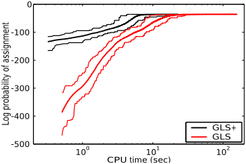
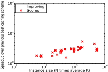
Figure 1: (a) Effect of the modification of the evaluation function in GLS+ compared to GLS on instance Munin2. Given are the best, average and worst solution quality over computation time for 25 runs of GLS and GLS+. The GLS+ plot ends after 22.94 CPU seconds when all its runs have found the optimal solution quality. (b) The speedup achieved by our new caching schemes over the previously best-performing caching scheme on a collection of randomly generated and real-world instances, where instance size is given as the number of variables (N) times the average domain size (K).
minimized is defined as g(v) = ∑φ∈Φ λφ[V = v], where λφ[V = v] is the penalty associated with solution component Vφ = vφ. It may be noted that this deviates from the standard form of the evaluation function for the general GLS algorithm, which also captures the contribution of each solution component to the optimisation objective p(v).
Due to this non-standard evaluation function, the sole interaction of objective function and penalties in Park's GLS for MPE is via the utilities of potentials φ under the current assignment v, which are defined as util(φ, v) = -φ[V = v]/(1 + λφ[V = v]). An entry φ[Vφ = vφ] with high probability is assigned low utility, and its associated penalty λφ[Vφ = vφ] will be increased less often, driving the search towards the partial variable instantiation Vφ = vφ eventually, but possibly only after a considerable delay.
Due to this initial and persistent lack of greediness, we expected the performance of GLS for MPE to be boosted significantly by integrating the objective function into the search heuristic. We achieved this by a change in GLS's evaluation function. Our improved version of GLS, which we call GLS+, adds the logarithmic objective function to the appropriate penalties, making the new evaluation function to be maximized g(v) = ∑φ∈Φ log(φ[V = v])-w×λφ[V = v], where w is a weighting factor. 3 Indeed, this modification of the evaluation function has major consequences on search behaviour and especially boosts the search in early phases of the search. Figure 1(a) illustrates this for the real-world network Munin2 (from the Bayesian Network Repository), where GLS+ finds optimal-quality solutions 10 times faster on average.
GLS+ differs from GLS in a number of other components, namely the parameter setting, the caching scheme, and the initialization. All of these modifications contribute significantly to GLS+'s improved performance (a detailed analysis of their individual importance can be found in [Hutter, 2004]). Firstly, a thorough experimental analysis showed that, although Park states that "GLS had no parameters to tune." [Park, 2002], its performance can be boosted by up to several orders of magnitude by simply changing Park's default smoothing value ρ = 0.8 to the constant value ρ = 0.999. For example, for the Hailfinder network GLS finds the optimal solution 10 times faster with ρ = 0.999 than with ρ = 0.8, and for several random instances this effect is much more pronounced. It is interesting to note that the very small amount of smoothing performed at ρ = 0.999 can be rather important: Without smoothing (ρ = 1), we found rare but conclusive evidence for search stagnation on random networks.
3 In order to achieve a meaningful guidance by this evaluation function in areas of the search space with probability zero, we treat log(φ[V = v]) as -104 for φ[V = v] = 0; we also fixed the weighting factor w to 104 to make the penalties comparably large.
Secondly, the subsidiary local search procedure in GLS uses a computationally efficient first-improvement strategy, whereas GLS+ employs a more powerful best-improvement procedure in conjunction with newly developed, powerful strategies for caching and updating the effects of variable flips on the evaluation function. While previously used caching schemes only locally update the partial evaluation function value involving variables in the Markov blanket of a flipped variable, we developed two substantial improvements. At every step, we maintain the score of flipping each variable to any of its values (caching scheme Scores), and on top of that the set of all variables that lead to an improvement in evaluation function value when flipped to some value (caching scheme Improving); since after an initial search phase this quantity is a low constant in practice, this latter caching scheme enables an evaluation of the whole neighbourhood of a search position in constant time. Figure 1(b) demonstrates the large performance gains of our new caching schemes over the previous state-of-the-art caching scheme.
Thirdly, GLS initializes the search randomly. However, it has been shown that strong initial solutions, such as the ones obtained with MB, lead to much better overall solutions [Kask and Dechter, 1999]. Consequently, GLS+ initializes its search using the MB variant MB-w(105 ) (see Section 2), which improves the quality of found solutions considerably and for some instances speeds up the search for optimal solutions by up to two orders of magnitude.
We also study a version of GLS+ that has an additional preprocessing stage based on VE. In this preprocessing, VE is applied until a potential with more than b entries is obtained, where b is a parameter (b = 0 results in the standard GLS+ algorithm, and b = ∞ yields pure VE). The resulting reduced network can then quickly be solved with GLS+, and the eliminated variables can be instantiated optimally in linear time like in regular VE.
| Distribution | Stats | GLS+ | GLS | BBMB | AOMB | |||
|---|---|---|---|---|---|---|---|---|
| W | Opt | (default) | (orig) | static(10) | dynamic(4) | static(10) | dynamic(6) | |
| Random networks | ||||||||
| Base-line: N = 100, K = 2, P = 2 | 16.5 | 100 | 0.11 | 1.88(1/0) | 0.05 | 1.69 | 0.33 | 1.10 |
| N = 200, K = 2, P = 2 | 34.8 | 0 | 0.70 | 33.97(68/0.8464) | 61.95(88/0.2694) | 47.66(86/0.4168) | -(100/0) | -(100/0) |
| N = 400, K = 2, P = 2 | 72.6 | 0 | 10.13 | -(100/0.0355) | -(100/0.0020) | -(100/0.0254) | -(100/0) | -(100/0) |
| N = 100, K = 3, P = 2 | 16.5 | 100 | 0.34 | 37.15(81/0.7392) | 5.51 | 28.90(7/0.5608) | 15.38 | 33.72(20/0) |
| N = 100, K = 4, P = 2 | 16.3 | 60 | 0.88 | -(100/0.2225) | 21.86(25/0.4856) | 29.88(65/0.5071) | 42.41(53/0) | 59.02(91/0) |
| N = 100, K = 2, P = 3 | 28.3 | 47 | 0.42 | 13.26(3/0.9659) | 36.12(48/0.3650) | 31.49(74/0.3884) | 43.01(62/0) | 53.17(62/0) |
| N = 100, K = 2, P = 4 | 37.0 | 0 | 0.81 | 41.89(4/0.8538) | 46.83(98/0.1079) | 2.07(99/0.1502) | -(100/0) | -(100/0) |
| Grid networks | ||||||||
| Base-line: N = 10, K = 2 | 11.8 | 100 | 0.01 | 4.55(5/0.1989) | 0.05 | 20.23(7/0.6847) | 0.13 | 2.56 |
| N = 15, K=2 | 22.4 | 0 | 0.90 | 50.00(99/0.4201) | 9.75(95/0.2686) | -(100/0.0880) | -(100/0) | -(100/0) |
| N = 20, K=2 | 32.8 | 0 | 30.01 | -(100/0.0031) | -(100/0.0058) | -(100/0.0015) | -(100/0) | -(100/0) |
| N = 25, K=2 | 44.3 | 0 | 52.06 | -(100/0) | -(100/0.0002) | -(100/0) | -(100/0) | -(100/0) |
| N=10, K = 3 | 12.0 | 100 | 0.34 | -(100/0.4955) | 0.98 | 47.16(97/0.3187) | 1.90 | 43.29(53/0) |
| N=10, K = 4 | 11.7 | 95 | 1.17 | -(100/0.0496) | 4.77(3/0.5950) | -(100/0.1830) | 15.59(4/0) | 68.32(95/0) |
| N=10, K = 5 | 11.8 | 84 | 5.05 | -(100/0.0098) | 6.41(9/0.5619) | -(100/0.1334) | 76.52(33/0) | -(100/0) |
| N=10, K = 6 | 11.9 | 0 | 17.89 | -(100/0.0049) | -(100/0) | -(100/0.0940) | -(100/0) | -(100/0) |
4 Experimental Results
We conducted a number of computational experiments to compare the performance and scaling behaviour for the original GLS algorithm, GLS+, and the current state-of-the-art in MPE solving. 4 In [Marinescu et al., 2003], B&B with static MB heuristic (s-BBMB) and a B&B algorithm with MB tree elimination heuristic (BBBT) were claimed to be the stateof-the-art for MPE solving. [Marinescu and Dechter, 2004] then introduced B&B with dynamic MB heuristic (d-BBMB), as well as versions of s-BBMB and d-BBMB that employ an AND/OR search tree; these are called s-AOMB and dAOMB.
We used Radu Marinescu's C++ implementations of sBBMB, d-BBMB, s-AOMB, and d-AOMB. 5 Furthermore, we used Marinescu's C++ implementation of GLS instead of the original Java implementation by Park [Park, 2002], since the former was orders of magnitude faster than the latter on all instances we tried; our GLS+ implementation is also written in C++. We employed a fixed parameter setting of 〈ρ,Nρ〉 = 〈0.999, 200〉 for GLS+ and the overall bestperforming fixed i-bound ib ∈ {2, 4, 6, 8, 10, 12} for each B&B algorithm. The preprocessing stage in GLS+ only improves its performance for structured networks. Thus, we set b = 0 in the experiments on random instances.
4 All experiments were carried out on compute servers each equipped with dual 2GHz Intel Xeon CPUs with 512KB cache and 4GB RAM running Linux version 2.4.20, build 28.9. Our implementation and the benchmark instances we used are available online at http://www.cs.ubc.ca/labs/beta/Projects/SLS4MPE/
5 We do not report results for BBBT, since the implementation available to us could only correctly handle networks generated within the REES system (http://www.ics.uci.edu/˜radum/rees.html).
In the first two experiments, for each network, we executed each algorithm once for a maximum of 100 CPU seconds and call the best solution found in any such run of an algorithm quasi-optimal. For the second and third experiment, we ran the B&B algorithms for a long time to obtain provably optimal solution qualities, which we found to always agree with our quasi-optimal solutions. For a fair comparison, we always report the times each algorithm requires for finding a quasioptimal solution; only for the third experiment we additionally report the time required for proving optimality. Finally, we define the approximation quality of an algorithm run as the ratio of the probability of the solution it found and the quasi-optimal probability.
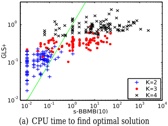
Our first experiment evaluates how the various algorithms scale with important instance characteristics, such as network size (N), domain size of the variables (K), and network density, here controlled by the number P of parents of each node. We created instances with a random network generator provided by Radu Marinescu (this is, e.g., described in [Marinescu et al., 2003]), topologically sampled all variables to guarantee non-zero joint probability, and randomly picked 10 evidence variables. Table 1 shows that for small and easy networks, identified as "Base-line" in the table, the original GLS and the B&B algorithms are competitive with GLS+, but that when scaling any of N, K, or P, the performance of all algorithms except GLS+ degrades rapidly. [Marinescu et al., 2003] showed that s-BBMB scales much better with domain size K than the original GLS algorithm. While this is confirmed by our experiments (see Table 1), our results in Figure 2(a) show that GLS+ substantially outperforms s-BBMB for larger K, and that the relative variability in run-time increases with K for s-BBMB, but remains constant for GLS+.
GLS+ does not only outperform the other algorithms in terms of runtime for finding quasi-optimal solutions, but also in terms of solution quality found in a given fixed time. This
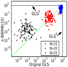
- (b) Approximation quality of GLS, GLS+, and s-BBMB(10)
(c) Scaling with induced width
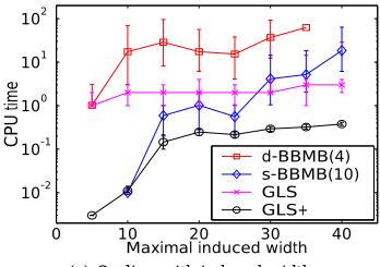
Figure 2: (a) CPU time required by GLS+ and s-BBMB(10) to solve random network instances to optimality. Each point is the result of a single run on one instance. The instances are the same as summarized in Table 1. The same CPU-time for both algorithms is indicated by the line. (b) Comparison of the quality reached by the three algorithms GLS, GLS+, and sBBMB(10) within 100 CPU seconds. For all instances, GLS+ found the best known solution quality, thus its approximation quality is always 1. Each point in the figure is the result of a single run for one instance by GLS and s-BBMB(10), while the two lines show the approximation quality of GLS+. (c) Scaling with induced width for random networks with 100 variables, domain size 2, and maximal node degree 5. For each induced width, based on one run on each of 100 instances, we plot the median runtime for finding the optimal solution. The errorbars are based on the quantiles q0.25 and q0.75. We do not employ means and standard deviations since the B&B algorithms did not succeed in finding an optimal solution for every network. For example, for the networks of induced width 40, GLS+ took 0.5 seconds in the worst case, whereas s-BBMB(10) failed to find the optimal solution for 18 of the 100 networks within 100 seconds.
can be seen from Table 1 for all of N, K and P, and is visualized in Figure 2(b) for scaling N in random grid networks. This scatter plot compares the original GLS, GLS+, and s-BBMB all given the same maximum computation time; this is possible since GLS+ always finds the quasi-optimal solutions, such that its approximation quality is constantly 1. Even though s-BBMB(10) scales better than the original GLS, GLS+ shows even better scaling behaviour. Once again, not only the average quality difference to GLS+ grows, but for both GLS and s-BBMB, the relative variability also increases with network size.
These scaling results are further extended in our second experiment, where we studied the impact of the induced width of networks on the performance of GLS+ vs. GLS and the B&B algorithms. For this, we used networks generated with BNGenerator, 6 which allows to generate networks with a rather accurate upper bound on the induced width. The results in Figure 2(c) show that the induced width has a major effect on algorithm performance, and that GLS and GLS+ scale much better with induced width than the B&B algorithms (we omit s-AOMB and d-AOMB which were worse than d-BBMB). We attribute this to the B&B algorithm's MB heuristic whose guidance is impaired for high induced widths.
In our third experiment we studied real-world networks from the Bayesian Network Repository. 7 Here, GLS+ also performs very well, except for large networks with low induced width, which are easily solved with VE. As we show in Table 2, a short preprocessing stage (b > 0) significantly improves the performance of GLS+ for these structured networks, making it faster than all B&B algorithms (with optimal i-bound) for all but one network. 8 In particular, note that the Link network could not be solved by any of the B&B algorithms, while GLS and GLS+ find the optimal solution in one CPU second. Interestingly, MB(2) already finds a tight upper bound on solution quality (in 10 CPU milliseconds), but with feasible i-bounds never even comes close to a tight lower bound. Consequently, only a combination of SLS and MB can find the optimal solution and prove its optimality (and this within one CPU second).
6 http://www.pmr.poli.usp.br/ltd/Software/BNGenerator/
7 http://www.cs.huji.ac.il/labs/compbio/Repository/
8 To study whether GLS+ eventually finds the optimum even
5 Conclusion and FutureWork
In this work, we identified various weaknesses of GLS, the previously best-performing SLS algorithm for the MPE problem, and introduced GLS+, a novel variant of GLS that pays more attention to such important concerns as algorithmic complexity per search step, thorough parameter tuning, and strong guidance by the evaluation function. For a wide range of MPE instances, GLS+ widely outperforms GLS and the best-performing exact algorithms (all of which are B&B algorithms) that defined the state-of-the-art in MPE solving. Most importantly, we demonstrated that the performance of GLS+ scales much better than GLS and B&B algorithms with the network and domain size, as well as with network density and induced width. GLS+ also shows the best performance for real-world instances.
In contrast to recent claims that stochastic local search algorithms are not competitive for MPE solving [Marinescu et al., 2003], our results establish SLS as a state-of-the-art approach for MPE solving that merits further investigation. In particular, the anytime characteristics and excellent scaling
without the preprocessing (b = 0), we performed 25 additional runs of two hours on the instances Diabetes and Munin4. Out of these, eleven runs solved the Diabetes network, but the Munin4 network was never solved. This highlights the importance of preprocessing for structured networks.
| Instance | Stats | GLS+ | GLS+ | Nrest | VE | GLS | BBMB | AOMB | |||||||||
|---|---|---|---|---|---|---|---|---|---|---|---|---|---|---|---|---|---|
| N | K | w | with b = 0 | optimal | b | (orig) | static | ib | dynamic | ib | static | ib | dynamic | ib | |||
| Barley | 48 | 8.77 | 7 | 19.22 | 17.95 | 104 | 31 | - | (-) | 2.58/2.58 | 6 | 6.28/68.91 | 4 | 3.08/3.08 | 6 | 43.37/43.37 | 4 |
| Diabetes | 413 | 11.34 | 4 | (0.0099) | 3.61 | ≥ 106 | 0 | 3.61/3.61 | (-) | 4.55/4.55 | ≥6 | - | - | 8.64/8.64 | ≥6 | 162.28/162.28 | 8 |
| Link | 724 | 2.53 | 15 | 1.25 | 1.16 | 102 | 352 | - | 1.0 | (0.0050) | 10 | (0.0050) | 4 | - | - | - | - |
| Munin1 | 189 | 5.26 | 11 | 0.34 | 0.34 | 104 | 45 | - | 1.0 | 1.25/10.57 | 6 | 1.03/45.84 | 4 | 6.42/6.42 | 6 | 38.15/38.15 | 4 |
| Munin2 | 1003 | 5.36 | 7 | 0.96 | 0.91 | 104 | 79 | 1.9/1.9 | 1.0 | 3.98/6.55 | 8 | 76.36/- | 6 | 2.77/2.77 | 6 | 10.24/40.24 | 8 |
| Munin3 | 1044 | 5.37 | 7 | 0.87 | 0.83 | 104 | 62 | 1.5/1.5 | (-) | 4.34/4.34 | 12 | 27.59/44.10 | 10 | 2.39/2.39 | 6 | 12.92/12.92 | 6 |
| Munin4 | 1041 | 5.43 | 8 | (0.0347) | 1.87 | 104 | 157 | 17.69/17.69 | (-) | 21.30/24.75 | 12 | (0.0090) | 4 | 20.77/20.77 | 8 | 128.24/128.24 | 8 |
behaviour of GLS+ suggest its use for large problems with real-time constraints, such as finding the MPE in pairwise MRFs for early computer vision [Boykov et al., 2001]. We therefore plan a comparative study of GLS+, generalized BP and graph cuts, which currently define the state-of-the-art in that domain [Tappen and Freeman, 2003]. Furthermore, in the near future we plan to implement an extension of GLS+ that computes a diverse set of high-quality MPEs-the SLS paradigm accommodates such an extension easily, for example, by using the best solutions encountered along the search trajectory.
Acknowledgments. We would like to thank Radu Marinescu for providing implementations of GLS and of several B&B algorithms, as well as code for the generation of Bayes nets. We also thank James Park for providing his original GLS code.
@inproceedings{ijcai2005p210,
  title     = {Efficient Stochastic Local Search for MPE Solving},
  author    = {Hutter, Frank and Hoos, Holger H. and Stützle, Thomas},
  booktitle = {Proceedings of the Nineteenth International Joint Conference on
               Artificial Intelligence, {IJCAI-05}},
  publisher = {International Joint Conferences on Artificial Intelligence},
  editor    = {Leslie Pack Kaelbling and Alessandro Saffiotti},
  pages     = {169--173},
  year      = {2005},
  url       = {https://ijcai.org/proceedings/2005/210},
}
TY - CPAPER TI - Efficient Stochastic Local Search for MPE Solving AU - Hutter, Frank AU - Hoos, Holger H. AU - Stützle, Thomas T2 - Proceedings of the Nineteenth International Joint Conference on Artificial Intelligence, IJCAI-05 PB - International Joint Conferences on Artificial Intelligence PY - 2005 SP - 169 EP - 173 UR - https://ijcai.org/proceedings/2005/210 ER -Copied
Machine-readable versions of this paper, for tools and AI agents:





