Representing Flexible Temporal Behaviors in the Situation Calculus

1 Introduction

In real-world domains robots have to perform multiple tasks either simultaneously or in rapid alternation, employing diverse sensing and actuating tools, like motion, navigation, visual exploration, mapping, and several modes of perception. To ensure a suitable multiple-task performance, some approaches (e.g. [14; 23]) have recommended that executive control processes supervise the selection, initiation, execution, and termination of actions. From these ideas, a new paradigm has been proposed, called the Constraint Based Interval Planning (CBI), which essentially amalgamates planning, scheduling and resources optimization for reasoning about all the competing activities involved in a flexible concurrent plan (see [10; 4; 7]). The CBI approach, and similar approaches emerged from the planning community, have shown a strong practical impact when it comes to real world applications (see e.g. RAX [10], IxTeT [7], INOVA [21], and RMPL [23]). However, from the standpoint of cognitive robotics it is important to ensure both optimal performance, in practical applications, and to provide a logical framework for ensuring coherence of actions preconditions and effects. The system coherence emerges as a core issue also when control processes negotiate resources allocation with individual perceptual-motor and cognitive processes; indeed, the executive has to establish priorities among individual processes to allot resources for multiple-task performance (see the discussion in [8; 11; 3]). Therefore, different, concurrent, and interleaving behaviors, subject to switching-time criteria and current situation needs, lead to a new integration paradigm. In this paper we suggest that the reactive aspects that have to cope with flexible behaviors and the cognitive capabilities enabling reasoning about these processes, can be combined in the Temporal Flexible Situation Calculus. We present a new approach to flexible behaviors, that exploits the full expressiveness of the Situation Calculus (SC) [19; 12], where computational concerns related to time can be monitored by a temporal network, obtained via a transformation of added constraints. To embed many concepts elaborated in the CBI framework we extend the SC with concurrency and time (extensions of SC with time was already explored in [15; 17; 16]), deploying Allen's interval relations [1], and further constraining the language to represent concurrent timelines. In this framework we can conjugate the advantages of the SC with the expressive power of the CBI paradigm. Our aim here is twofold: on the one hand, it is made possible to introduce a separated timeline for each component of the dynamic system (i.e. each entity, which is part of an autonomous system, such as a robot), so that concurrency and flexibility can be clearly addressed; on the other hand the causal relationships among processes can be dealt with in the SC language, which provides a clear framework for preconditions and postconditions of actions and a simple solution to the frame problem. We show that the CBI perspective, with all its arsenal of specifications in terms of flexible time, alternation constraints, resources optimization, failure recovering, and tasks scheduling, can be imported into the SC ([19; 12]), defining a temporal and concurrent extension of the basic action theory (related approaches are [15; 17; 16; 8; 20; 6]). Finally, we provide a version of the Golog language and interpreter for manipulating flexible plans on multiple timelines.

2 Preliminaries

2.1 Situation Calculus and Golog

The Situation Calculus [12; 19] is a sorted first order language for representing dynamic domains by means of actions, situations, and fluents. Actions and situations are first order terms, and situation-terms stand for history of actions, compound with the binary symbol do: do(a, s) is the situation obtained by executing the action a after the sequence s. The dynamic domain is described by a Basic Action Theory BAT = (Σ, DS0 , Dssa, Duna, Dap). We refer the reader to [19] for a complete introduction to the SC. Temporal Concurrent Situation Calculus (TCSC) has been earlier introduced in [15; 18; 17]; actions are instantaneous, and their time is selected by the function time(.). Durative actions are considered as processes [15; 19], represented by fluents, and durationless actions are to start and terminate these processes. For example, going(hill, s) is started by the action startGo(hill, t) and it is ended by endGo(hill, t′ ).

Golog. Golog is a situation calculus-based programming language for denoting complex actions composed of the primitive (simple or concurrent) actions defined in the BAT. Golog programs are defined by means of standard (and not so-standard) Algol-like control constructs: i. action sequence: p1; p2, ii. test: φ?, iii. nondeterministic action choice p1|p2, iv. conditionals, while loops, and procedure calls. An example of a Golog program is:

The semantics of a Golog program δ is a SC formula Do(δ, s, s′ ) meaning that s′ is a possible situation reached by δ once executed from s. For example, Do(a;p, s, s′ ) .= Do(p, do(a, s), s′ ) ∧ Poss(a, s) defines the execution of an action a followed by the program p. For more details on the SC and Golog we refer the reader to [19].

2.2 Constraint Based Interval Paradigm

The constraint based interval framework (CBI) [10; 4], is a well known framework for temporal planning systems combining temporal reasoning and scheduling, including, e.g., RAX [10], IxTeT [7], and INOVA[21]. The CBI paradigm accounts for concurrency and time, and action instances and states are described in terms of temporal intervals linked by constraints. We refer to the timeline-based version of the CBI [10] where a domain behavior is seen as the continuous interaction of different components, and each component is represented by state variables; a single state variable is a relevant feature of the components and represents a concurrent thread. Both states and activities are uniformly treated as temporal intervals. The history of states for a state variable over a period of time is called a timeline. Figure 1 illustrates two timelines (state variables) repr. the engine and the navigation processes of a mobile robot: initially, the robot is at(p1) and stop; when it starts go(p1, p2) the engine is running; the engine is stop again once the rover arrives at(p2). Some temporal constraints among the activities are: at(x) holds only if stop holds, go(x, y) is followed by at(y).

Domain Constraints. A CBI model [10] Mcbi=(X, J,R) is defined by: i. a set X={x1, . . . , xn} of state variables, one for each component (e.g. xloc and xeng in Fig. 1); ii. a set J = {J1, . . . , Jn} s.t. for each xi the set Ji collects the associated temporal fluents pi,j(⃗y), e.g. at(x) and go(x, y) for location state variable in Fig. 1; iii. a set of temporal constraints R={ri,j}, usually called compatibilities: for each temporal fluent property pi,j there is a compatibility relation ri,j representing all its possible legal relations with the other temporal fluents, i.e. which temporal property must proceed, follow, be co-temporal, etc. to pi,j in a legal plan. The latter are specified in terms of metric version of temporal relations a la Allen [1]. E.g. the arrows in Fig. 1 illustrate the compatibility associated to the fluent at: at(x) meets go(x, y), and at(x) during stop.

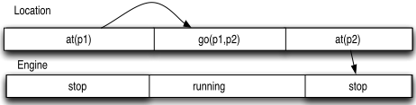
Planning Problem in CBI. Given the CBI model Mcbi, a planning problem is defined by Pcbi = (Mcbi, Pc), where Pc is a candidate plan, representing an incomplete instance of a plan. The candidate plan defines both the initial situation and the goals. In particular, Pc consists of : i. a planning horizon h; ii. a set of temporal properties to be satisfied for each state variable xi ∈ X (e.g. at(p1) ends before 10 and after 20 in the timeline of Figure 1); iii. the set of precedence constraints among fluents pk,1 ≺ pk,2, which are to hold on a timeline, e.g. at(p1) ≺ at(p2); iv. the set of constraints R={ri,j} associated with the temporal properties pi,j mentioned in the timelines. A fluent pi,j(⃗x) mentioned in a candidate plan is fully supported [10] if all its associated constraints ri,j are satisfied. E.g. in Figure 1 at(p1) and at(p2) are fully supported. A candidate plan is said to be a complete plan if: i. each temporal property on each timeline is fully supported; ii. all timelines fully cover the planning horizon. Given the planning problem (Mcbi, Pc), the planning task is to provide a sufficient plan [10], i.e. a complete plan with the maximum flexibility: the planner is to minimally ground the (temporal) variables to allow for on-line binding of the values.

3 Temporal Flexible Situation Calculus

In this section we present the Temporal Flexible Situation Calculus framework (TFSC), which integrates the CBI paradigm, introduced above, into the language of SC.

Actions. We define a partition {αv; v ∈ C} of the set of actions according to the different components C the system has to care of. For example, the component Pan-Tilt-Unit manages actions like start-scan spts(.), or end-scan epts(.). To induce the partition we introduce a type operator ν, and extend the SC foundational axioms with the following definitions. Let H = ⋃ni=1 Hi be a set specifying the types of actions, we assume this set finite. For each name of action the following holds:

Hi(a)∧Hj(a′ )→¬(a = a′ ) for i̸=j, and ν(A(⃗x))=ν(A′ (⃗y)) ≡ ∨ni=1 Hi(A(⃗x)) ∧ Hi(A′ (⃗y)), together with the unique name for actions, here the indices stay only for different components names, a denotes an action variable, while A denotes the name of an action function.

Situations. Typization of actions induces also a partition on the set of situations whence on the set of histories. Histories become streams of situations over timelines. Typization is inherited by situations as follows:

For each component v ∈ C, a timeline is specified by a history of actions concerning v. The evolution of the set of timelines is a set of situations sc = {sv|v ∈ C}, called situation class, spanning different types. In other words, ∃s.s ∈ sc abbreviates: ∃s1 . . . sn ∃a1 . . . an. ∨ni=1 [s = do(ai, si)∧ ν(ai) = ν(si)∧ ∧nj=1,i̸=j ν(ai) ̸= ν(sj)]. Where ν(si) is the type of situation si corresponding to some component i ∈ C, n=|C|. The sc class is equipped with the following ≤c relation:

do(av, sc) denotes the sequence resulting from adding the action av to a type-compatible situation mentioned in sc.

Time. Time is part of the sorted domain of TFSC, as noted in Section 2; we extend the time selection function from actions to situations (see [16] for a different notation), and situation classes as follows:

The time of a situation class sc, depends on the time of the situations in sc, so time(sc) = t abbreviates:

Consistency of the extension. The above axioms concerning types, time and situation classes, are added to the foundational axioms in Σ and are conservative (i.e. obtained by extending the language), therefore the extended set (which we still denote with Σ) must be consistent.

Processes. Processes span the subtree of situations, over a single interval specified by a start and end action. They are implicitly typed by the actions process: for each process there are two actions, starting and ending the process, abbreviated by sP , meaning starts process P and eP , meaning ends process P . A process is denoted by a fluent P (⃗x, t-, s), (here tis its start time). Successor state axioms (SSP) for processes extend the set of SSA for fluents and are defined as follows:

For example, moving towards θ, can be defined as:

Action preconditions axioms define the conditions for the start and end actions to be executed. Let P be a process, we say that it is linear if it does not mention any other process in the right-hand side of the definition. The set Dssp of successor state axioms for processes is linear if all processes mentioned in it are linear. Let Dssp be a set of linear successor state axioms for processes, let the BAT be D ∪Dssp = Σ∪DS0 ∪Duna ∪Dss ∪DAP ∪Dssp then:

Proof (sketch). The proof relies on the relative consistency of the SC. Furthermore, linearity of Dssp ensures that there are no loops w.r.t. time, hence for each start and end action, as defined in the processes, it is not possible to introduce dependencies that could lead, for instance, to sP (⃗x, t) < sQ(⃗y, t′ ) and sP (⃗x, t) > sQ(⃗y, t′ ).

Intervals. Intervals mention temporal variables, which are always free, and get assigned only according to a specified set of behaviors, in so being very well suited for representing flexible behaviors. In this paragraph we show how embedding intervals in the SC leads to the construction of a temporal network. The following formula Ψ, specifies the conditions for a process Pi to hold on its induced timeline, from t-i to t+i with arg. x:

Let p,m, o, d, s, f, e abbreviate the usual precedes, meets, overlaps, during, starts, finishes, equals, as defined in the temporal intervals literature, started in [1], with op ranging over all relations, and let γop denote:

We represent the interval relations between processes, given in situation-suppressed form (i.e not mentioning situations), and taking the "end-time" t+ as argument, according to the following macro-definition, where the free variables mentioned in Ψi (see (6) above) are just hidden:

Note that the metrical version (like in [10]) including durative relations can be analogously defined. Letting each operator in the macro being not commutative, inverse can be defined as Pi op-1 Pj = Pj op P1.

We assume that the domain theory DT is associated with temporal relations, as those given in (7), specifying the temporal interactions between processes as constraint patterns. For example, wanting to say that going has always to be preceded by beingAt we would associate to DT the set {going([t-g , t+g ]) p beingAt([t-b , t+b ]). We call this set the temporal compatibilities abbreviated by Tc.

We denote I(τ, sc) the set of the (7) interval relations associated with the situation class sc, where τ is the set of time variables, varying over the intervals [t+, t-], related to the set of timelines sc. The I(τ, sc) is obtained by abducing the time constraints on τ, according to a construction illustrated in the paragraphs below. For instance, for a suitable sc and τ = {[t-1 , t+1 ], [t-2 , t+2 ], [t-3 , t+3 ], [t-4 , t+4 ]} we can get the set:

whose constraints are depicted in the network of Fig. 2.

Temporal Constraint Network. The satisfiability problem we are concerned with is the following. Let DT = D∪Dssp∪ I(τ, sc) be a basic theory of actions, extended with time specifications (see eq. (3) above), successor state axioms for processes, time interval constraints, in which time variables are free, and with an associated set of compatibilities Tc. We seek an assignment set for time variables, which is a feasible solution for the constraints, and s.t. a substitution of the free variables for this set induces an interpretation, which is a model of DT ∪ I(τ, sc). To find such an assignment we appeal to the concept of general temporal constraint networks (TCN) introduced in Meiri [13] following the one developed for discrete constraint networks [5]. A TCN involves variables denoting both intervals and points, together with unary and binary constraints. A TCN is associated with a direct constraint graph where each node is labeled by a temporal variable and labeled-directed edges represent the binary relations between them (e.g. p, e etc.). According to the underlying temporal algebra, TCNs express different forms of reasoning (Allen's interval algebra [1], the Point Algebra [22], metric point algebra [5], and so on) see in particular [2]. Let τ = {X1, . . . ,Xn} = {[t-1 , t+1 ], . . . [t-n , t+n ]} be a set of time variables, denoting intervals (i.e. each variable Xi denotes an interval [t-1 , t+1 ]), and let R be a set of binary relations; the assignment set V = {[s1, e1], . . . , [sn, en] : si, ei ∈ R, si < ei} is called a solution set for R, if {X1 = [s1, e1], . . . , Xn = [sn, en]} satisfies all the constraints defining R. The network is consistent if at least one solution set exists. In the sequel we shall identify a TCN with its labeled direct graph and denote with V a solution set. We also say that V satisfies the constraints.

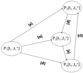
Mapping SC to TCN. Let h : I(τ, sc) ↦→ TCN, h(I(τ, sc)) is a temporal network Net, with cardinality m, specified by the nodes labeled by the defined processes {Pi, Pj |PiopPj}, mentioned in I(τ, sc).

By the above definitions the network Net is consistent if there exists an assignment V to the temporal variables τ, which is a feasible solution for I(τ, sc). For example the set V={[10, 160], [10, 70], [75, 95], [95, 150]} is a solution set for the variables τ={[t-1 , t+1 ], [t-2 , t+2 ], [t-3 , t+3 ], [t-4 , t+4 ]}, of the network depicted in Figure 2, given the relations {m, p, d, s, f}. Note that, in the macro definition (7), there are two parts, the left-hand component is the definiendum Pi(x, t-i , t+i ) op Pj(x, t-j , t+j ), which is mapped into a temporal network, while the right-hand component is the definiens Ψi→(Ψj ∧γop)[τ ], which is interpreted into a structure of the SC, where the assignments for the free temporal variables τ are obtained by the TCN. A semantic correspondence, between the network and the formulae of SC, can be established as follows. Let M=〈D, I〉 be a structure of SC (where D is a sorted domain and I an interpretation) we extendMwith the above defined mapping h, i.e. Mh=〈D, I, h〉. ThenMh is a model for D∪I(τ, sc), iff there is a consistent temporal network h(I(τ, sc)), under some assignment V to the free time-variables, satisfying I(τ, sc). Given the above definitions we can state the following:

Lemma 2 Let DT be a consistent action theory. DT ∪ I(τ, sc) is consistent iff there exists a consistent temporal constraint network h(I(τ, sc)), under the assignment V , such thatMh, V |= ∧ D∧Ψ[τ].

Proof(sketch). Let h(I(τ, sc)) be a consistent temporal network, under the assignment V . Consider the formula Ψ[τ ] =, ∧i,j≤m Ψi→(Ψj∧γopij ), with τ the set of free time-variables in Ψ, and we let M be a model for DT . M can be extended to a model for all the γopij according to V , as follows. For each process Pi build a chain of situations of the kind Γi = {do(sPi (t′i ), σ′ ) ≤ σ ≤ do(ePi (t′′ i ), σ′′ ) ≤ σi}, with σ a sequence such that ePi is not mentioned in σ, and the free-temporal variables are from τ according to the Pi timeline in sc. Extend the structure M to one for DT ∪ ⋃i Γi by choosing from V a suitable assignment to the free variables τ , appearing in each Γi, and according to the constraints in the γopij , corresponding to those in I(τ, sc), and such that each sequence is satisfied. This is always possible, because each process is made true of a situation by a start action, and false by an end action, by the sequence construction, on a timeline. Then V is an assignment to τ s.t. (Mh, V ) is a model for DT ∪ ⋃i Γi[τ]. Finally it is enough to show that any model for DT ∪ ⋃i Γi[τ], is a model for Ψ[τ]. ✷

By Lemma 1 DT ∪ I(τ, sc) is consistent iff DS0 ∪ I(τ, sc) is consistent. Logical implication can be now defined as follows. Let Mh = 〈D, I, h〉, and β(τ ) be a formula with all its free temporal variables among τ :

TCN construction. The TCN construction involves the following inference mechanisms: i. abduce I(τ, sc) to obtain the temporal network topology h(I(τ, sc)); ii. implement the temporal constraints into situations, according to the network. We show the inference process through an example. Let Tc = {P1 m P2}, be the compatibilities specified in the domain theory. Let sc = do([sP1 (t-1 ), eP1 (t+1 ), sP2 (t-2 ),eP2 (t+2 ), sP1 (t′1-), eP1 (t′1+)], S0), then the abduced constraints, according to Tc, sc and τ , are:

From the above constraints a three nodes network h(I(τ, sc)) would be constructed. The time range of the solutions to the network - given the free temporal variables and the situation class sc - is a flexible situation class, which is a triple of the kind 〈sc, τ, i〉, where i(τ) is the constraint over the freevariables, e.g. i(τ) = 7 ≤ t-1 ∧ t+2 > 10.

Progression. Wewant to determine if, according to the timing and advancements of the current situation class, we can forget about past scheduled processes and think of future resources allocation. This is the well known progression problem [19] in the SC. We face here a simplified version of the progression problem, and with regressable formulas, which is all we need. Let us state the problem as follows. Given a sentence ϕ, one needs first to determine the set of situations in sc to which it can be progressed, given the timelines, and a candidate interval t = [t-, t+]. To this end one has to order the situation terms in ϕ according to the relation ≤sc introduced in (2), and get the smallest situations set, w.r.t. ≤sc, mentioning t; let it be min. We now consider the domain theory Dmin T , which is equal to DT but with DS0 replaced by a set W min = {ϕ|DT |= ϕ}, where ϕ mentions only ground situations σ, with {σi}=scmin, but no free variables of sort time. Let Φ(t1, . . . tn) be a SC formula mentioning situations {σi} ≥sc min, which are ground but for possible free variable of sort time all among t1, . . . , tn. Then

Proof. (sketch) One direction follows by cut. For the other direction, suppose DT ∪ I(τ, sc) |= Φ(t1, . . . , tn), let us regress Φ(t1, . . . , tn) along the different timelines, this can be done by separating Φ into a DNF, and considering each conjunct separately, we regress it with respect to min, and let G be the regressed formula - note that no change is needed in regression to account for regressed sentences as time variables will be kept as they are, without turning to quantified variables through successor state axioms (as they are universally quantified in linear Dssp). Then by definition of W min , G ∈ W min hence, by the previous lemma, the claim follows.

4 Flexible High Level Programming in Golog

Golog Syntax. Given the extended action theory presented above, the following constructs inductively build Golog programs:

1. Primitive action: α.
2. Nondeterministic choice: α|β. Do α or β.
3. Test action: φ?. Test if φ is true in the current sit. class.
4. Nondet. arg. choice: choose ⃗x for prog(⃗x).
5. Action sequence: p1; p2. Do p1 followed by p2.
6. Partial order act. choice: p1 ≺ p2. Do p1 before p2.
7. Parallel execution: p1‖p2. Do p1 concurrently with p2.
8. Conditionals: if φ then p1 else p2.
9. While loops: while φ do p1.
10. Procedures, including recursion.

Golog Semantics. The macro Do(p, sc, sc′ , h) gives the semantics for the above constructs; where p is a program, sc and sc′ are situation classes, and h specifies the finite horizon.

• Null program:

• Primitive first program action with horizon:

Here, if the first program action is applicable to si ∈ sc, and ai can be scheduled after the horizon then it is neglected (i.e. each action, which can be started after the horizon can be postponed).

• Partial order action choice:

Here, either the second program can be directly executed, or it is possible to insert a primitive action a, selected by a suitable fluent predicate select(a, s) representing the selection criterion (set to true if no selection holds).

• Parallel execution:

• Test action:

Here φ[sc] stands for generalization of the standard φ[s] in the SC extended to situation classes, e.g. P1[sc] ∧ P2[sc] is for P1(s1)∧P2(s2) with s1, s2 ∈ sc, i.e. each fluent is evaluated w.r.t. its specific timeline.

• The semantics of nondet. action choice, nondet. argument selection, conditionals, while loops, and procedures is defined in the usual way.

Flexible Temporal Behaviors inGolog. The CBI planning problem (Mcbi, Pc) introduced in Section 2.2 can be easily coded and solved in the TFSC framework. Given a DT representing the timelines and processes in Mcbi, a candidate plan Pc can be encoded by a Golog program progc. This is possible once we introduce, for each interval constraint for pi,j(⃗r) in Pc, a Golog procedure of the kind:

where ψj i is the macro (6) associated with the process P j i (i.e. i-th process in the j-th timeline), and γ any temporal constraint. For example, go(d, e) ends in [6, 10] can be represented as

Given the πi,j procedures, a partial specification of a single timeline Tj can be easily defined using the ≺ operator:

Given a set of timelines {Ti}, a candidate plan Pc can be represented as a parallel execution of the plan Ti:

Since a CBI complete plan P is associated with a fully supported set of timelines {T i} and a set of constraints i(τ) (see Section 2.2), we can introduce a mapping g transforming a CBI plan P into a flexible situation 〈sc, τ, i〉. The following holds.

Proposition 1 Given a CBI planning problem (Mcbi, Pc), where Pc is a candidate plan [10], for any complete plan P of (Mcbi, Pc), maximally flexible in the time variables τ, there exists a DT , a Golog program progc, where

with 〈sc, τ, i〉 a flexible situation, and such that:

The proof is omitted.

Example. We assume an autonomous rover, which has to explore the environment and perform observations. While the robot is moving the pant-tilt unit must be pointing ahead ptIdle. To point to a location x the rover must be stopped there, at(x), while the pan-tilt scans in direction z: ptScan(x, z). Hence, we consider two components: pant-tilt, navigation. Each component has a set of processes: Jpt={ptIdle, ptScan(z, x)}; Jnav={at(x), go(x, y)}. Each of these is to be encoded in the DT as in (5), e.g. ptScan(t, z, x, do(a, s)) ≡ a = spts(z, x, t) ∨ptScan(t, z, x, s) ∧ ¬∃t′ .a = epts(z, x, t′ ). The temporal compatibilities Tc among the activities are defined by a set of temporal constraints patterns, defined by macros (7), e.g.:

go(x, y, t1, t2) m at(y, t3, t4); at(x, t1, t2) m go(x, y, t3, t4); go(x, y, t1, t2) d ptScan(z, x, t3, t4); ptScan(z, x, t1, t2) d at(x, t3, t4).

Consider a partial specification for the rover behavior: from time 0 to 3 it must remain at(p1), and at time 0 the pant-tilt is ptIdle; the rover mission is to observe p3, in direction θ before 30 and after 20, and be back at p1 before 50. This candidate plan, can be encoded in the following Golog program:

proc(mission, ψnav at (p1, 0, 3)? ≺ (ψnav at (p1, t11, t12) ∧ t12 ≤ 50)? : Nil‖ ψpt pti (0, t21)? ≺ (ψpt pts (θ, p3, t22, t33) ∧ [t22, t23] ⊆ [20, 30])? ≺ Nil).

Given the horizon h = 50, and an initial situation class ini, a possible complete plan is a flexible situation 〈sc, τ, i〉, with sc[τ]={σnav[τ1], σpt[τ2]}, s.t. DT ∪ I(τ, sc) |= Do(mission, ini, sc[τ ], 50), e.g.

σnav=do([sat(p1, 0), eat(p1, 3), sgo(p3, t11), ego(p3, t12), sat(p3, t13), eat(p3, t14), sgo(p1, t15), ego(p1, t16)], S0); σpt=do([spti(0), epti(t21), spts(t22), epts(t23), spti(t24), epti(t25), s]S0),

and i(τ) is the minimal set of constraints solving the h(I(sc, τ)) temporal network, i.e. {t12 = t13 < t14 = t15 < t16 < 50; t21 = t22 < t23 = t24 < t25; t22 > t13, t23 < t14 }.

Implementation. We provided a constraint logic programming (CLP) [9] implementation of the Golog interpreter. Since the Golog interpreter is to generate flexible temporal plans, it must be endowed with a constraint problem solver. Analogous to [17] we rely on a logic programming language with a built-in solver for linear constraints over the reals (CLP(R)). We appeal to the ECRC Common Logic Programming System ECLIPSE 5.7. Currently, we are deploying the Golog interpreter as the control engine of a monitoring systems for robotics applications.