
Combining Learning Constraints and Numerical Regression
Proceedings of the Nineteenth International Joint Conference on Artificial Intelligence. Pages 596-601.
© 2005 International Joint Conferences on Artificial Intelligence
Abstract
Usual numerical learning methods are primarily concerned with finding a good numerical fit to data and often make predictions that do not correspond to qualitative laws in the domain of modelling or expert intuition. In contrast, the idea of Q2 learning is to induce qualitative constraints from training data, and use the constraints to guide numerical regression. The resulting numerical predictions are consistent with a learned qualitative model which is beneficial in terms of explanation of phenomena in the modelled domain, and can also improve numerical accuracy. This paper proposes a method for combining the learning of qualitative constraints with an arbitrary numerical learner and explores the accuracy and explanation benefits of learning monotonic qualitative constraints in a number of domains. We show that Q2 learning can correct for errors caused by the bias of the learning algorithm and discuss the potentials of similar hierarchical learning schemes.
- [Atkeson et al., 1997] C.G Atkeson, A.W Moore, and S.A. Schaal. Locally weighted learning. Artificial Intelligence Review, 11:11-73, 1997.
- [Blake and Merz, 1998] C.L. Blake and C.J. Merz. UCI repository of machine learning databases, 1998.
- [Breiman et al., 1984] L. Breiman, J.H. Friedman, R.A. Ol- shen, and C.J. Stone. Classification and Regression Trees. Wadsworth, Belmont, California, 1984.
- [Dietterich, 1998] T.G. Dietterich. Machine-learning re- search: Four current directions. The AI Magazine, 18(4):97-136, 1998.
- [Domingos, 2000] Pedro Domingos. A unified bias-variance decomposition and its applications. In Proc. 17th Interna- tional Conf. on Machine Learning, pages 231-238.
- Mor- gan Kaufmann, San Francisco, CA, 2000.
- [Gama and Brazdil, 2000] J. Gama and P. Brazdil. Cascade generalization. Machine Learning, 41(3):315-343, 2000.
- [Geman et al., 1992] S. Geman, E. Bienenstock, and R. Doursat. Neural networks and the bias/variance dilemma. Neural Computation, 4(1):1-58, 1992.
- [Kuipers, 1994] B. Kuipers. Qualitative Reasoning: Mod- eling and Simulation with Incomplete Knowledge. MIT Press, Cambridge, Massachusetts, 1994.
- [Quinlan, 1993] J.R. Quinlan. Combining instance-based and model-based learning. In Proceedings of the 12th In- ternational Conf. on Machine Learning, pages 236-243, San Mateo, CA, 1993.
- Morgan Kaufmann.
- [Stone and Veloso, 2000] P. Stone and M. Veloso. Layered learning. In Machine Learning: ECML 2000 (Proceedings of the 11th European Conference on Machine Learning), pages 369-381. Springer Verlag, 2000.
- [Todorovski and Džeroski, 2003] L. Todorovski and S. Džeroski. Combining classifiers with meta deci- sion trees. Machine Learning, 50(3):223-249, 2003.
- [Šuc and Bratko, 2002] D. Šuc and I. Bratko. Qualitative re- verse engineering. In Proceedings of the 19th Interna- tional Conf. on Machine Learning, pages 610-617.
- Mor- gan Kaufmann, 2002.
- [Šuc and Bratko, 2003] D. Šuc and I. Bratko. Improving nu- merical accuracy with qualitative constraints. In Proceed- ings of the 14th European Conference on Machine Learn- ing, pages 385-396. Springer, 2003.
- [Šuc et al., 2004] D. Šuc, D. Vladušič, and I. Bratko. Qual- itatively faithful quantitative prediction. Artificial Intelli- gence, 158(2):190-219, 2004. IJCAI
- [Šuc, 2003] D. Šuc. Machine Reconstruction of Human Con- trol Strategies, volume 99 of Frontiers in Artificial Intel- ligence and Applications. IOS Press, Amsterdam, The Netherlands, 2003.
- [Witten and Wang, 1997] I.H. Witten and Y. Wang. Induc- tion of model trees for predicting continuous classes. In Proc. Poster Papers Europ. Conf. Machine Learning, 1997.
- [Wolpert, 1992] D.H. Wolpert. Stacked generalization. Neu- ral Networks, 5(2):241-259, 1992.
References were extracted automatically from the PDF and may contain errors.
Full text extracted automatically from the PDF; figures, tables and equations may differ. The PDF is the version of record.
1 Introduction
Learning understandable models is one of the main goals of machine learning, but has been recently overshadowed by methods that mainly concentrate on classification or regression accuracy. Less effort has been devoted to improving the explanation strength of machine learning methods. Induced models are often too complex and overly detailed to provide an understandable explanation of phenomena in a modelled domain. This is particularly notable with methods that achieve excellent accuracy by constructing ensembles of classifiers (overview in [Dietterich, 1998]). Another problem, illustrated and discussed in [ ˇSuc et al., 2004], is that state-ofthe-art numerical machine learning methods often make predictions that a knowledgeable user finds obviously incorrect
- not so much in numerical, but in qualitative terms. Such qualitative errors of numerical predictors are undesirable particularly because they make numerical results difficult to interpret. The underlying mechanism in the domain is usually best explained in qualitative terms. However, this is obscured by qualitative errors in numerical predictions.
Qualitatively faithful quantitative learning, called Q 2 learning for short, was proposed [ˇSuc et al., 2004] to rectify the qualitative problems of numerical learning. Q 2 learning combines qualitative and numerical learning to give numerical predictions that both fit the data well and are consistent with an induced qualitative model. The qualitative consistency is beneficial in terms of explanation of phenomena in a modelled domain. Quite surprisingly, a case study with Q 2 learning shows that induced qualitative constraints can also improve numerical accuracy. This paper extends the previous work in several directions.
One contribution of this paper is a Q2 learning scheme that combines learning of monotonic qualitative constraints with an arbitrary numerical learner and enables us to study accuracy benefits of the induced constraints. Qualitative learning has been previously used in a number of applications that are mainly tied to dynamic systems and control. In these applications, advantages in terms of explanation and in terms of the control performance of the induced qualitative models were observed. Since these models define only constraints on a class variable, a direct assessment of their accuracy benefits was previously not possible. The second contribution is an empirical evaluation in a number of domains and a demonstration that such regression, guided by induced qualitative constraints, often increases numerical accuracy.
We analyze the reasons for these accuracy improvements and show that Q2 learning corrects for errors caused by the bias of a learner. In this respect Q2 learning is similar to ensembles of classifiers, in particular approaches that combine classifiers constructed by different learning algorithms, e.g. combining instance and model-based learning [Quinlan, 1993] or stacking and its variations [Wolpert, 1992; Gama and Brazdil, 2000; Todorovski and Dˇzeroski, 2003 ]. An important distinction of Q2 learning is the (qualitative) consistency of models at different levels of abstraction. We discuss advantages of similar hierarchical learning schemes and we demonstrate that explanation improvements do not necessarily come at the price of lower accuracy.
In Section 2 we describe the Q2 learning scheme proposed in this paper. The elements and the details of Q 2 learning are described in Section 3. Then we give experimental results in various domains and study accuracy improvements using bias-variance decomposition. Section 5 discusses results and benefits of Q2 learning, and gives directions for future work.
2 Q2 Learning with QUIN and Qfilter
The idea of Q2 learning is to combine qualitative and numerical learning to find a regression function that fits the data well and is consistent with an induced qualitative model. In this paper, Q2 learning consists of two stages:
- Program QUIN 1 (described in Section 3.1) induces a qualitative tree from numerical training examples. Qualitative trees are similar to decision trees, but have monotonic qualitative constraints in their leaves.
- AlgorithmQfilter (described in Section 3.2) uses the induced qualitative tree, plus training examples, plus class predictions of an arbitrary numerical learner, to alter the predictions to respect the induced qualitative tree. Qfilter is an optimization procedure that finds the minimal quadratic changes in class values that achieve consistency with the qualitative tree. In our experiments, the numerical learners, also called base-learners, are regression trees, model trees and locally weighted regression.
In this paper, a Q2 learner consists of a qualitative constraints learner and a numerical base-learner, and can be denoted by Q2 (qual-learner, base-learner). We abbreviate the common case Q2 (QUIN, base-learner) simply as Q2baselearner. This learning scheme is particulary interesting because base-learner's predictions are changed optimally in the sense of squared error. Therefore, the differences between base-learner's predictions and Q2 predictions come just from induced qualitative constraints.
3 Elements of Q2 Learning
3.1 Monotonic Qualitative Constraints, Qualitative Trees and QUIN
Monotonic qualitative constraints (MQCs) are a kind of monotonicity constraints that are widely used in the field of qualitative reasoning and are a generalization of monotonic function constraint used in QSIM [Kuipers, 1994]. A simple example of an MQC is: Y = M +(X). This says that Y is monotonically increasing in its dependance on X, i.e. whenever X increases, Y also increases. In general, MQCs can have more than one argument. For example, Z = M +,-(X, Y ) says that Z is monotonically increasing in X and monotonically decreasing in Y . If both X and Y increase, then according to this constraint, Z may increase, decrease or stay unchanged. In such a case, an MQC cannot make an unambiguous prediction of the qualitative change in Z.
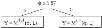
Qualitative trees are similar to decision trees, but have monotonic qualitative constraints in the leaves. Figure 1 gives an example of a simple qualitative tree. This qualitative tree is a qualitative model of the function Y = Lsin(Φ), where 0 ≤ Φ ≤ π and L > 0. It describes how Y qualitatively depends on attributes Φ and L. The tree partitions the attribute space into two regions that correspond to the two leaves of the tree. Note that a simple qualitative tree can describe a relatively complicated nonlinear function. Such qualitative trees are induced from numerical data by learning program QUIN [ ˇSuc, 2003].
1 QUIN with a graphical user interface, Qfilter and locally weighted regression as a base-learner are available at http://ai.fri.uni-lj.si/dorian/q2/quin.htm.
QUIN constructs a qualitative tree in a top-down greedy fashion, similar to decision or regression tree learning algorithms. The split selection criterion is based on the minimum description length principle and takes into account the encoding complexity of the subtrees, the consistency of the MQCs in the subtrees with the corresponding data, and the "ambiguity" of the MQCs with respect to the data (the more unambiguous qualitative predictions the MQC can make, the better).
3.2 Qfilter Algorithm
Qfilter handles each leaf of a qualitative tree separately. It first splits the examples according to the qualitative tree and then changes class values to achieve consistency with MQCs in corresponding leaves.
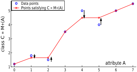
Let us first observe a simple example in Figure 2. We have eight examples (ai, ci), i=0, 1, ..., 7. Class C has values ci and attribute A has values ai=i. The examples are not consistent with the given MQC C =M +(A), because the MQC requires that ci+1 > ci which is violated at i = 1 and i = 4.
To achieve consistency with C = M +(A), class values should be changed into ci + di, where the unknown parameter di denotes the change in the i-th class value. Class changes di are constrained by MQC-imposed inequalities: ci+1 + di+1 > ci + di where i = 0, 1, ..., 6. These inequalities can be formulated in matrix notation as Ad > b, where d is a vector of unknown parameters di, vector b has elements bi = ci - ci+i, and matrix A has elements ai,i = -1, ai,i+1 = 1 and zeros elsewhere. In general, b and A depend on the MQC-imposed inequalities, which in turn depend on the MQC and on the ordering of attributes' values.
Therefore, finding minimal quadratic changes in class values that achieve consistency with a given MQC can be posed as the quadratic programming optimization problem: find vector d that minimizes the criterion function d T H d such that Ad > b. In the above formulation matrix H is the identity matrix. In general H can be changed to differently penalize the changes in class values as described in Section 3.3.
Since the criterion function with diagonal matrix H is a convex function, and because the linear constraints Ad > b define a convex hull, a local minimum of the criterion function is a globally optimal solution. A more elaborate description of Qfilter, defining also the appropriate ordering of class values when more than one attributes are used in an MQC, is given in [ˇSuc and Bratko, 2003]. In previous work Qfilter was used with qualitative trees derived manually from domain knowledge. Here we use it in a different and a more challenging context, where qualitative trees are induced from data.
3.3 Qfilter for Q2 Learning
Qfilter is supplied with a qualitative tree, training examples with their class values and test examples with the baselearner's class predictions. Qfilter then adjusts the class values of the training and the test examples to achieve consistency with the qualitative tree.
One improvement of Qfilter is to use the base-learner's confidence estimates in its predictions. In this case, Qfilter makes smaller adjustments to the class values with higher confidences at the expense of larger changes of class values that have lower confidences. This is achieved by changing the quadratic programming criterion function. Namely, matrix H is changed from the identity to a diagonal matrix with elements hi,i = wi. Weight wi is computed from the base-learner's confidence estimate in the i-th class value. Of course, the computation of weight wi depends on a type and a scale of confidence estimates, but would generally be larger if a numerical predictor is more confident in the i-th class prediction.
Based on this idea, we used a heuristic weighting function: wi = 1+sign(µ-ci)(1-exp ( -(ci-µ)2 2σ )), where ci denotes base-learner's confidence in the class prediction of the i-th test example, and µ and σ denote the mean and the standard deviation of base-learner's confidences over all test examples. Therefore, the weight of a test example is between zero and two. The weight of all training examples is set to two. In experiments with locally weighted regression, confidence estimates ci were set to the sizes of confidence intervals. Model and regression trees do not provide similar confidence estimates. For this reason, confidence estimates of all test examples were set to one.
4 Empirical Evaluation
4.1 Experimental Details
Here we evaluate accuracy benefits of Q2 learning with various numerical base-learners. Given a set of training examples, a base-learner is used to predict class values of test examples. The same training examples are used for QUIN to induce a qualitative tree. The qualitative tree, the training and the test examples with base-learner's class predictions are then used by Qfilter to give predictions that are consistent with the qualitative tree. This procedure is then repeated (for example, ten times with ten-fold cross-validation) with different training and test examples.
In the experiments we compare root relative squared errors (RREs for short) of the base-learner and the Q 2 learner. Here, the RRE is the root mean squared error normalized by the root mean squared error of average class value. The baselearners in our study are regression and model trees [Breiman et al., 1984; Quinlan, 1993], and locally weighted regression [Atkeson et al., 1997]. The first two base-learners were chosen because they are well-established numerical learners that provide a symbolical model. Locally weighted regression (LWR for short) does not provide a model explaining a studied domain, but often gives more accurate predictions than model or regression trees. With such base-learners, the explanation benefits of Q2 learning are even more obvious. In experiments we used our implementations of these baselearners. Our regression and model trees use cost-complexity pruning [Breiman et al., 1984] and smoothing. LWR uses Gaussian weighting function with local optimization to set the kernel size at each prediction point. We also give RREs of M5 model trees [Quinlan, 1993] and its Weka implementation called M5Prime [Witten and Wang, 1997] to show that we are not comparing Q2 to base-learners that perform poorly. With all learners, default values of their parameters were used.
We analyze the reasons for the Q2 accuracy improvements using bias-variance decomposition [Geman et al., 1992] and draw some interesting conclusions.
4.2 Robot ArmDomain
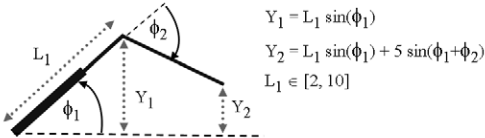
Here we describe experiments in the domain of a planar twolink, two-joint robot arm depicted in Figure 3. The angle in the shoulder joint is denoted by Φ1 and the angle in the elbow joint is denoted by Φ2. Angle Φ1 is between zero and π, while Φ2 is between -π/2 and π/2. The first link, i.e. the link from the shoulder to the elbow joint, is extendible with length L1 ranging from 2 to 10. The second link has fixed length 5. Y-coordinates of the first and the second link ends are denoted by Y1 and Y2 respectively. We experimented with four learning problems that differ in class variable (Y1 or Y2) and the attributes used for learning. These learning problems were defined to pose increasingly more difficult problems to Q2 learning.
| LWR | Q2LWR | Mt | Q2Mt | Rt | Q2Rt | M5Pr | |
|---|---|---|---|---|---|---|---|
| A | 0.187 | 0.145 | 0.264 | 0.238 | 0.327 | 0.293 | 0.512 |
| B | 0.196 | 0.139 | 0.159 | 0.146 | 0.318 | 0.263 | 0.462 |
| C | 0.327 | 0.300 | 0.336 | 0.324 | 0.434 | 0.378 | 0.489 |
| D | 0.403 | 0.362 | 0.366 | 0.363 | 0.542 | 0.448 | 0.553 |
The easiest learning problem, called problem A, is to predict the y-coordinate of the first link end given its length and angle, i.e. learning Y1 = f(L1, Φ1). Other learning problems require predicting the y-coordinate of the second link end using different attributes. In learning problems B and C we helped the learners with a derived attribute Φsum = Φ1+Φ2, i.e. the deflection of the second link from the horizontal. Problem C is to learn Y2 = f(L1,Φ1,Φ2,Φsum), while in problem B we also used Y1 as an attribute. Problem D requires learning Y2 = f(L1,Φ1,Φ2). These problems pose increasingly more difficult problems to Q 2 learning. The easiest is problem A, because a correct qualitative model is a simple qualitative tree, given also in Figure 1. Learning problem D is the most difficult for Q2 , since a correct qualitative model cannot be expressed by a qualitative tree.
To compare accuracy of different base-learners and Q 2 learning we generated examples where angles Φ1 and Φ2 and link length L1 were randomly generated from a uniform distribution. We experimented with different percentages of Gaussian noise in the class variable. Noise percentage p% means that the standard deviation of noise is p × dc/100, where dc denotes the difference between maximal and minimal class value. We used 100 training examples and measured accuracy on separate test sets of 200 examples without noise. All results are averages on 20 randomly generated training and test sets.
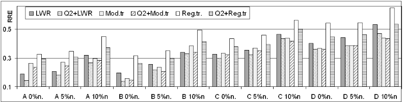
Table 1 gives RREs of LWR, model and regression trees and Q2 learning that uses these base-learners. For comparison RREs of M5Prime model trees are also given. Results with zero, 5%, and 10% noise are given in Figure 4. In all of the learning problems and with all noise levels, Q 2 improves the average RREs of all base-learners. These improvements in accuracy depend on the base-learner and the learning problem. Generally, the improvements are the greatest with regression trees and the smallest with model trees. It is notable that in general our base-learners are much more accurate than M5Prime on these learning problems. Although we are here not interested in comparison of different base-learners, it is good to know that with Q2 we are not improving the baselearners that performpoorly.
The significance of the Q2 accuracy improvements for each learning problemwas tested using the resampled paired t test. Four learning problems × three base-learners × three noise levels gives 36 comparisons of RRE of a base-learner and a corresponding Q2 learner. At 5% significance level, the Q2 learners are significantly better in 33 comparisons and about the same in only three comparisons. The comparisons where differences in RRE are not significant correspond to model trees on learning problem D with all three noise levels.
Bias-Variance Decomposition
To understand the reasons for the Q 2 accuracy improvements we used bias-variance decomposition [Geman et al., 1992; Domingos, 2000], which has proved to be a very useful tool for understanding machine learning algorithms. Biasvariance decomposition in regression states that the expected squared error of a learner on test example x is the sum of the irreducible noise N(x), the bias B(x) and the variance V (x). The bias B(x) of the learner on an example x is the squared difference between the true value and the mean prediction on x over all possible training sets. Here defined bias B(x) is in the literature called also squared bias, but we use the notation from [Domingos, 2000] and call it bias. The variance V (x) is the expected value of the squared difference between the true value and the mean prediction on x. The bias measures the systematic error incurred by a learner, and the variance measures the error incurred by its fluctuations around the central tendency in response to different training sets. Irreducible noise is the error of the optimal (Bayes) model and is in general very difficult to estimate. However, we are here using an artificial learning problem and can therefore measure the bias and variance by directly simulating the definitions.
We used 100 training sets of size 100, generated as in the previous experiment and measured the average bias and average variance on a test set of 810 equidistant data points. We refer to these averages over different training sets and different test examples simply as bias and variance. Comparing the base-learners we noticed that regression trees have the highest variance. This is in accordance with their complexity - they usually had more than 20 leaves. Model trees are smaller and have the smallest variance when no noise, but with increasing noise the variance increases most notably. Comparing Q 2 learners to the corresponding base-learners we noticed that Q2 always notably reduces the bias of the base-learners. This happens in all four learning problems, with all three baselearners and different noise levels. For example, in problem D with no noise, Q2 reduces bias and variance of LWR from 3.85 and 2.57 to 2.13 and 1.99, respectively. Q 2 always notably decreases the variance of regression trees, but sometimes increases the variance of LWR and model trees. The base-learners, used here, have a bias towards linear models. It seems that Q2 , with less restrictive monotonicity constraints, reduces their bias, but does not considerably increase the variance.
| Data set | Cases | Attributes | LWR | Q2LWR | Mod.tr. | Q2Mod.tr. | Reg.tr. | Q2Reg.tr. | M5 |
|---|---|---|---|---|---|---|---|---|---|
| AutoMpg | 398 | 5/8 | 0.361 | 0.380 | 0.374 | 0.386 | 0.459 | 0.405 | 0.383 |
| AutoPrice | 159 | 16/16 | 0.380 | 0.346 | 0.523 | 0.364 | 0.435 | 0.381 | 0.402 |
| Housing | 506 | 12/13 | 0.373 | 0.363 | 0.422 | 0.358 | 0.532 | 0.454 | 0.431 |
| MachineCpu | 209 | 6/6 | 0.353 | 0.317 | 0.370 | 0.334 | 0.460 | 0.377 | 0.414 |
| Servo | 167 | 2/4 | 0.478 | 0.457 | 0.588 | 0.584 | 0.508 | 0.504 | 0.536 |
| CraneSkill1 | 354 | 3/3 | 0.142 | 0.065 | 0.194 | 0.086 | 0.091 | 0.049 | 0.247 |
| CraneSkill2 | 618 | 3/3 | 0.249 | 0.169 | 0.190 | 0.159 | 0.191 | 0.165 | 0.215 |
| AntiSway | 200 | 4/4 | 0.414 | 0.157 | 0.319 | 0.250 | 0.193 | 0.165 | 0.412 |
Q2 learning combines hypotheses of two different learning algorithms, i.e. a qualitative learner and a numerical learner. In this respect it is similar to ensembles of classifiers and in particular approaches that combine classifiers constructed by different learning algorithms, as for example stacking and its variations. Such methods improve accuracy mainly by reducing the error due to the bias of a learner. This is the consequence of combining hypotheses that make uncorrelated errors [Dietterich, 1998]. We believe that such uncorrelated errors lead to bias reductions also in the case of Q 2 learning. It should be noted that, although Q 2 predictions are consistent with an induced qualitative model, they combine both the base-learner's predictions, and the qualitative model.
4.3 UCI and Dynamic Domains
To explore the potentials of learning similar constraints with a wider range of learning problems we describe experiments with eight data sets. The first five are the smallest regression data sets from the UCI repository [Blake and Merz, 1998] with the majority of continuous attributes. A reason for choosing these data sets is also that Quinlan [1993] gives results of M5 and several other regression methods on these data sets, which enables a better comparison of Q 2 to other methods. These data sets are AutoMpg, AutoPrice, Housing, MachineCpu and Servo.
The other three data sets are from dynamic domains where QUIN has typically been applied so far [ˇSuc, 2003; ˇSuc and Bratko, 2002]. It should be noted that in these domains the primary objective was to explain the underlying control skill and to use the induced qualitative models to control a dynamic system. Until now, it was not possible to measure their numerical accuracy or compare it to other learning methods.
Data sets CraneSkill1 and CraneSkill2 are the logged data of two experienced human operators controlling a crane simulator. Such control traces are typically used to reconstruct the underlying operator's control skill. The learning task is to predict the velocity of a crane trolley given the position of the trolley, rope angle and its velocity. Data set AntiSway was used in reverse-engineering an industrial gantry crane controller. This so-called anti-sway crane is used in metallurgical companies to reduce the swing of the load and increase the productivity of transportation of slabs. The learning task is to learn the control force applied to the trolley, given the desired and the current trolley velocity and the position and velocity of the load relative to the trolley.
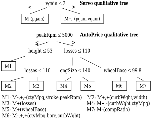
In all experiments, qualitative trees were considerably simpler than other induced models. Figure 5 gives examples of qualitative trees induced in data sets Servo and AutoPrice. These qualitative trees are considerably simpler than model trees. In Servo, M5Prime induces a model tree with eleven leaves, with all four attributes appearing in all eleven linear models. In AutoPrice, M5Prime induces a model tree with ten leaves, with at least ten attributes in each linear model.
Ten-fold cross-validation results are given Table 2. For each data set we give, respectively, the numbers of cases, numbers of continuous and all attributes, RREs of baselearners and RREs of corresponding Q 2 learners. The last column gives published RREs of M5 model trees [Quinlan, 1993] on UCI data sets, and RREs of M5Prime for others. These results are presented also in Figure 6.
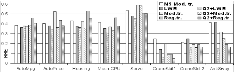
A general observation is that Q2 improves RREs of all three base-learners in seven out of eight data sets. Q 2 is worse just in AutoMpg with LWR and model trees. Smaller root relative squared errors in the last three data sets do not imply that these learning problems are easier, but are just the consequence of the normalization of RREs with large class variances.
The significance of the Q2 accuracy improvements was tested using the 10-fold cross-validated paired t test. Eight data sets × three base-learners gives 24 comparisons of RRE of a base-learner and the corresponding Q 2 learner. At 5% significance level, the Q2 learners are significantly better in 18 comparisons and about the same in six comparisons. The differences are not significant in AutoMPG with all three base-learners and with one base-learner in AutoPrice, Housing and CraneSkill2. Q2 is never significantly worse.
5 Discussion and Conclusions
The goal of this paper is to explore the accuracy and explanation benefits of Q2 learning that were observed also in previous work [ ˇSuc et al., 2004]. We extend the empirical evaluation to a number of domains and analyze the results. The proposed Q2 learning scheme, makes it possible to combine learning of qualitative constraints with an arbitrary numerical learner. It uses algorithmQfilter, which is particulary interesting since the base-learner predictions are optimally changed (in the sense of squared error) to be consistent with an induced qualitative tree. Therefore, the accuracy improvements of Q2 with respect to a base-learner are only due to the induced qualitative trees.
Q2 learning as a hierarchical learning scheme
Q2 learning, as presented in this paper, can be seen as a hierarchical learning scheme, where a learner at a higher level induces a hypothesis hn that guides the learner at a lower level. At higher levels of the scheme more abstract concepts (or more general constraints) are learned. In this way, hn provides inductive bias for learning of hypothesis hn-1. In the case of Q2 learning, h1 is a qualitative tree induced by QUIN and h0 are numerical predictions found by Qfilter. Similar hierarchical learning schemes were proposed either to improve the generalization of a single learning task, for example Stacked Generalization [Wolpert, 1992] and Cascade Generalization [Gama and Brazdil, 2000], or to facilitate the learning of several tasks in a hierarchy [Stone and Veloso, 2000]. Q2 learning has two distinctive properties. First, the hypotheses in the hierarchy are consistent and described at different levels of abstraction. This is important for the explanation of the phenomena in the modelled domain. Second, the hypotheses are learned in the general-to-specific order, which can reduce the search space, and can consequently improve also the generalization properties.
Explanation and Accuracy Benefits of Q2 Learning
Q2 predictions are consistent with a qualitative model that provides an explanation at a higher level of abstraction. In this respect Q2 learning is different than other methods for combining classifiers. Qualitative consistency enables Q 2 to improve numerical accuracy by combining hypotheses induced by different learners, but retain a simple explanation.
Benefits of qualitative learning in terms of providing simple and understandable explanations in various domains, including CraneSkill1, CraneSkill2 and AntiSway are discussed in [ˇSuc, 2003; ˇSuc and Bratko, 2002]. For example, qualitative trees induced in CraneSkill1 and CraneSkill2 have only a few leaves and were, because of their simplicity, preferred over the previous approaches for skill reconstruction, which typically learned regression or model trees with more than twenty leaves. Although the induced qualitative trees are simple, they reveal some surprising and nontrivial aspect of the human skill. Simple and understandable models were induced also in other domains studied in this paper. For example, in robot arm domain (problems A, B and C) QUIN usually induced qualitative trees that are very close to the correct qualitative models even with high percentage of noise. Simple qualitative trees were induced also fromUCI data sets (see Figure 5).
In the presented experiments, Q2 typically improved accuracy of the three base-learners. We compared root relative squared errors, but similar improvements were observed also with mean absolute errors. We experimented also with k-nearest-neighbor algorithm as a base-learner. It generally performed worse than the other three base-learners and the accuracy improvements of Q2 learning were even more obvious.
Bias-variance decomposition in the robot arm domain shows that the accuracy improvements stem mainly from correcting for errors caused by the bias of a base-learner. Experiments in the previous section suggest that combining "monotonic regularities" inductive bias with inductive bias of other learners is beneficial in a wide range of domains, also in domains when this might be less expected. As noted in Section 4.2, Q2 learning is similar to ensembles of classifiers, in particular approaches that combine classifiers constructed by different learning algorithms. Although, the accuracy improvements of Q2 are not comparable to those achieved by ensembles of classifiers, Q2 has advantages in terms of explanation.
Limitations and Future Work
Limitations of Q2 learning presented in this paper are mainly tied to the current implementation of QUIN. Because of its complexity it is difficult to apply it to very large data sets. Incorporating sampling techniques with qualitative learning might be beneficial. Another idea for future work is to assess and use the quality of the inducedMQCs in leaves, for example on a separate set of examples. The error of a Q 2 learner could be used to prune a qualitative tree. This might be useful also in data sets such as AutoMpg, where Q2 otherwise has problems. By considering only leaves where MQCs significantly improves a base-learner, a qualitative tree could be transformed into a set of qualitative association rules.
An interesting direction for future work is to explore the possibilities of the proposed hierarchical learning scheme with several layers of constrains, describing hypotheses at different levels of abstraction. Experimental results with Q 2 learning suggest that such scheme can be used to combine classifiers and improve accuracy, and, at the same time provide an understandable explanation of the phenomena in a modelled domain.
Acknowledgements
The work reported in this paper was supported by National ICT Australia and the Slovenian Ministry of Education, Science and Sport. National ICT Australia is founded by the Australian Government's Backing Australia's Ability initiative, in part through the Australian Research Council.
@inproceedings{ijcai2005p207,
  title     = {Combining Learning Constraints and Numerical Regression},
  author    = {Suc, Dorian and Bratko, Ivan},
  booktitle = {Proceedings of the Nineteenth International Joint Conference on
               Artificial Intelligence, {IJCAI-05}},
  publisher = {International Joint Conferences on Artificial Intelligence},
  editor    = {Leslie Pack Kaelbling and Alessandro Saffiotti},
  pages     = {596--601},
  year      = {2005},
  url       = {https://ijcai.org/proceedings/2005/207},
}
TY - CPAPER TI - Combining Learning Constraints and Numerical Regression AU - Suc, Dorian AU - Bratko, Ivan T2 - Proceedings of the Nineteenth International Joint Conference on Artificial Intelligence, IJCAI-05 PB - International Joint Conferences on Artificial Intelligence PY - 2005 SP - 596 EP - 601 UR - https://ijcai.org/proceedings/2005/207 ER -Copied
Machine-readable versions of this paper, for tools and AI agents:





