Lifted First-Order Probabilistic Inference

1 Introduction

Probabilistic inference algorithms are widely employed in artificial intelligence. However, most of them do not accept first-order specifications of models, which can abstract over classes of objects, requiring instead propositional ones which are longer and redundant because they must be specified variable by variable.

In the last decade, many proposals for algorithms accepting first-order specifications have been presented [Ngo and Haddawy, 1995; Ng and Subrahmanian, 1992; Jaeger, 1997; Kersting and De Raedt, 2000; Friedman et al., 1999; Pfeffer et al., 1999; Poole, 1993; Anderson et al., 2002; Richardson and Domingos, 2004; Laskey, 2005], most of which based on the theoretic framework of [Halpern, 1990]. However, these solutions perform inference at a mostly propositional level, that is, dealing with the random variables instantiated from the first-order, parameterized variables in the first-order specification (usually only the relevant random variables will be present in the propositional version). In domains with a large number of objects this may be both costly and essentially unnecessary. For example, a medical application can be about a large population of people infected with a certain disease and have a model of the probability of death of a person (any person) with that disease. To answer the query "what is the probability that someone will die of this disease?", an algorithm that depends on propositionalization would have to instantiate a random variable per patient. However this is not necessary since one can reason about individuals on a general level, provided one knows the population size, in order to answer that query in a much shorter time.

In such a scenario it would be possible to devise a way of using the available model to answer the query without considering each individual. However, this would require a manual devising of a process specific to the model or query in question. What is missing to date is an algorithm that can receive a general first-order model and automatically answer queries like these without computional waste.

A first step in this direction was given by [Poole, 2003], which proposes a generalized version of the variable elimination algorithm ([Zhang and Poole, 1994]) that is lifted, that is, deals with groups of random variables at a first-order level. The algorithm receives a specification in which parameterized random variables stand for all of their instantiations and then eliminates them in a way that is equivalent to, but much cheaper than, eliminating all their instantiations at once.

The algorithm in [Poole, 2003], however, works only for a very particular type of model because its only elimination operation is what we call inversion elimination, which requires special conditions explained later. These special conditions may sometimes be met by carefully chosen elimination orderings, but in certain cases no such ordering exists and inversion elimination cannot be applied at all steps. This introduces the need for another type of elimination, counting elimination, which can always be applied but costs more. By putting these two operations together we present the first algorithm capable of dealing with any first-order probabilistic model that operates directly on first-order representations, without resorting to a propositional level. We also show that the algorithm is correct and provide experimental results comparing it to a propositional algorithm.

2 Motivation

A probabilistic model over a set of random variables is defined by a set of dependencies, each of them on a subset of those variables. In a propositional model, each dependency explicitly refers to the variables it affects. For example, consider a Markov network involving a potential function, or factor, such as:

In fact, this type of potential function will be common enough in this paper that we define "if α then β p" to mean

where α and β are boolean formulas on binary random variables and V ar(α, β) is the set of these random variables. If p is omitted, it is assumed to be 1. "β p" is the same as "if ⊤ then β p" and "if α then β p else q" stands for both "if α then β p" and "if ¬α then β q". So we can write a model in the more readable fashion: 1

if epidemic then sick 0.7 if sick then death 0.4

In most practical problems, the same factor holds on many different sets of variables, requiring propositional models to repeat that factor several times, modulo the specific variables involved each time. In our example, if we wish to keep track of whether each member of a population is sick (with distinct variables sick(john), sick(mary), . . . ), we would have to write

if epidemic then sick(john) 0.7 if sick(john) then death(john) 0.4 if epidemic then sick(mary) 0.7 if sick(mary) then death(mary) 0.4 . . .

This renders the model specification unnecessarily complex and redundant. Moreover, an inference algorithm will consider each of those factors separately, even though there is some structure across them that should be exploited.

Currently, the most common way of dealing with these situations is to keep the original model and use it for each separate object (in this case, each person) as needed. This however does not help when different instances of the factor need to be used at the same time, as it would be the case to answer the query P(sick(john) ∧ sick(mary)), for example. In these situations, procedures specific to a given model have to be manually tailored, in what is a time consuming solution.

A natural way around this problem is to specify recurring factors in a parameterized way. This would allow us to express the same as above in the more succint way

if epidemic then sick(Person) 0.7 if sick(Person) then death(Person) 0.4

where Person (and, in our notation, words starting with a capital) is a typed logical variable assuming any value from the set of people involved in the problem. The semantics of this representation is simply that it should be equivalent to the propositional model formed by all possible instantiations of its logical variables. Following [Poole, 2003], we call these parameterized factors parfactors.

1 The reason we define the model with this "conditional" potential function rather than with usual conditional probabilities is that we concern ourselves with Markov networks (undirected models) only in this paper.

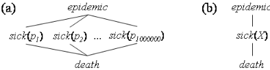
This semantics immediately provides an inference algorithm for such a representation, namely the one in which we apply any regular propositional inference algorithm to the propositionalized model, but this would be overkill. For example, in order to solve the query P(death(john)|sick(john)) it is only necessary to consider the instantiations for Person = john, ignoring other values. One could also consider general queries such as P(sick(Person)|death(Person)) that do not require any instantiations at all in order to be solved. An extreme example of the benefit of directly using the first-order representation is given by adding the parfactor "if death(Person) then someDeath" to the model and considering the query P(someDeath|epidemics). The tree width of the propositionalized graphical model is the population size, while the query can in fact be answered in time independent from the population size (a similar example is shown in fig. 4). It is therefore desirable to have an algorithm performing lifted inference, that is, inference directly on the first-order level, which instantiates parfactors only when necessary.

The languages we mentioned before allow parameterized specifications of probabilistic models. However, no corresponding first-order inference algorithm has been provided; inference is still performed by generating some propositionalized form of the model and using regular propositional inference algorithms on them (although some systems, like SPOOK in [Pfeffer et al., 1999], benefit from the first-order structure in some ways). In this paper we present an algorithm which performs exact lifted inference on first-order models.

It is also useful to allow deterministic constraints on the logical variables of parfactors. For example,

diabetes(P erson) 0.01, P erson ̸ = john ∧ P erson ̸ = mary

The constraint Person1 ̸ = Person2 in the first factor states that only its instantiations satisfying this condition will be considered. In the second factor, the potential of 0.01 for the random variable diabetes(Person) is assigned only for instantiations in which Person is distinct from john and mary.

3 Language, notation and semantics

Our language and semantics are essentially the same as those in [Poole, 2003], that is, those of a Markov network specified in a first-order language that allows parameterized random variables, 2 and are also similar to Markov logic networks [Richardson and Domingos, 2004]. A parfactor is a triad (φ,A,C) representing the applications of a potential function φ on all instantiations of a tuple of logical atoms A according to assignments to the logical variables in these atoms that satisfy a constraint formula C. At this point, we restrict ourselves to constraints with a finite number of solutions so as to have finite models only (this prevents us from using function symbols - more on this in section 6). For example, (1) is represented by the parfactor (φ, A, C), where φ is the appropriate potential function, A is {sick(P erson1),roommate(P erson2), sick(P erson2)} and C is Person1 ̸ = P erson2.

2 Poole discusses some aspects of directed models, however.

Note that we are in no way committed to the "if . . . then" construction used, which is simply a notation for a specific type of potential function. Any potential function is allowed, and random variables can be multivalued rather than binary only.

Just as with regular undirected graphical models, here the joint probability distribution is determined by the product of all potential functions given an assignment to all random variables (which are instantiations of atoms in parfactors, and therefore ground atoms). The only difference is that in a first-order model this product involves all instantiations of all parfactors. Given a set of parfactors G, the joint distribution defined by it is

where RV (G) is the set of all random variables (ground atoms) involved in all instantiations of all its parfactors, Θg is the set of all assignments, or substitutions, to the logical variables of g that satisfy its constraint (the solutions to the constraint), φg is the potential function in g, Ag is the tuple of atoms in g and Agθ is the instantiation of this tuple given an assignment θ to logical variables.

Further notation include, for a parfactor g, Cg for the constraint in g and, for a set of parfactors G, AG for the atoms in G, CG for the total constraint ∧ g∈G Cg and ΘG for the set of solutions of CG. For any object α, LV (α) and RV (α) are the sets of logical and random variables in α, respectively. Finally, all sets of parfactors are implicitly assumed to be standardized apart, that is, logical variables are renamed if necessary so that no logical variable is used in more than one parfactor in the set.

4 Inference

The inference problem is, given a set of random variables (ground atoms) Q representing a query, to calculate the marginal probability of Q given a model G (queries involving a condition can be issued by adding parfactors representing this condition to G). This is

where ∑RV (G)\Q is a summation over all assignments to random variables not in Q and φ(G) is a shorthand notation for the right-hand side of equation (2).

Calculating this summation by brute force is intractable, but one can use independencies in the model to do it more efficiently. In propositional models, one way of doing this is

PROCEDURE FOVE(G, Q)

G a set of parfactors, Q a set of random variables (the query).

1. If RV (G) = Q, return G.
2. G← SHATTER(G,Q) (figure 2).
3. E ←FIND-ELIMINABLE(G,Q).
4. GE ← {g ∈ G : RV (g) and RV (E) intersect}.
5. G¯E ←G \GE.
6. g ′ ←ELIMINATE(GE,E).
7. G ′ ← {g ′ } ∪G¯E.
8. Return FOVE(G ′ ,Q).

PROCEDURE FIND-ELIMINABLE(G, Q)

G a set of parfactors, Q ⊂ RV (G), G shattered against Q.

1. Choose e fromAG \Q.
2. Ge ← {g ∈ G : RV (g) and RV (e) intersect}.
3. If LV (e) = LV (Ge) ({e} is inversion-eliminable) return {e}.
4. Return FIND-COUNT-ELIMINABLE(G,Q, {e}).

PROCEDURE ELIMINATE(G, E)

G a set of parfactors, E ⊂ RV (G).

1. A ′ ←AG \E.
2. g ← (a0 g∈G φ |ΘG|/|Θg| g ,A ′ ,CG) (fusion, section 4.4).
3. If LV (E) = LV (g) (E is inversion-eliminable) return parfactor (✁ e φg(A ′ θ, e), A ′ , Cg).
4. Return

( ✁ N1 · · · ✁ Nu N1! . . .Nn! a0 k i φg(vi,A ′ ) |Vi| ,A ′ ,⊤) (as detailed in section 4.3).

PROCEDURE FIND-COUNT-ELIMINABLE(G, Q, E)

G a set of parfactors, Q ⊆ RV (G), E ⊆ AG \ Q.

1. If AGE \ E is ground (E is counting-eliminable) return E.
2. Choose a non-ground atom e ∈ AG \ E.
3. Return FIND-COUNT-ELIMINABLE(G,Q,E ∪ {e}).

Figure 1: First-order variable elimination algorithm.

the variable elimination (VE, [Zhang and Poole, 1994]) algorithm which calculates the total marginal by dividing it into smaller partial marginalizations, each on a single variable. The main contribution of this paper is a first-order version of VE, FOVE, which is shown in Figure 1 and works in a similar way by eliminating one (but maybe more) atoms and their respective constraints at each step. The advantage of FOVE is that, by eliminating an atom with its associated constraints, we are effectively eliminating all of its groundings in a lifted way, with a cost that is sometimes independent of the number of groundings.

4.1 FOVE correctness

We now show that FOVE is correct. The algorithm works in the following way: suppose we want to eliminate the atoms in a set E at a given step of it. Then we can write

where RV (E) is the set of random variables resulting from all instantiations of E in G, GE is the subset of parfactors in G depending on RV (E), and G ¯E is G \ GE.

If we can represent ∑RV (E) φ(GE) as the potential of a single parfactor g ′ , (defined such that φ(g ′ ) = ∏θ∈Θg φg(Agθ)), we can reduce the original marginal ∑RV (G)\Q φ(G) to a marginal on a model G ′ = G ¯ E ∪ {g ′ } which involves fewer random variables:

There are two ways, described below, of calculating a parfactor g ′ such that φ(g ′ ) = ∑RV (E) φ(GE): (1) inversion elimination or (2) counting elimination. (1) is the preferable one because it does not depend on the number of objects in the domain or, in other words, the size of RV (E). However, this method requires certain conditions on E (explained later) that may be impossible to satisfy for any E in the atoms of G. (2) is less favorable as it depends on the size of RV (E) (it is still better than propositionalization, though), but it is always possible to find an E on which it can be applied.

In the two next subsections, we assume that GE has been replaced by an equivalent parfactor g. This operation is called fusion and is explained in section 4.4. We are thus left with the problem of expressing ∑RV (E) φ(g) as a parfactor.

Finally, we assume that the parfactors and query have been shattered, as explained in section 4.5. The main property of shattered parfactors and query is that any two atoms in them have groundings which are either identical or completely disjoint. Why this matters will be explained as inversion and counting elimination are explained.

4.2 Inversion elimination

Inversion elimination assumes that E is a unary set {e} such that LV (e) = LV (g), where LV (α) is the set of logical variables in α. Let θ1 . . . θn be an enumeration of Θg. Then

(because of shattering)

for g ′ a new parfactor (φ ′ ,A ′ ,Cg) where A ′ is a tuple of the atoms distinct from e in Ag, φ ′ (A ′ θ) = ∑eθ φg(Agθ), and Cg is the constraint formula of g.

Note that the initial sum of products becomes a product of sums, hence the name inversion elimination. Also note that the sum providing φ ′ is over the assignments on the parameterized random variables. Therefore this elimination method does not depend on the number of groundings, but on the number of assignments to the parameterized random variable, which is much smaller.

The condition LV (e) = LV (g) is essential for this method to work because it guarantees that the random variables being summed out have a one-to-one correspondence to the instantiations of g. This is a condition not taken into account by [Poole, 2003], whose method eliminates all random variables not in the query by inversion elimination, one by one. However, the proof above should make it clear that this is not always possible. A numerical contradiction can be found by trying to answer the query r for p(X) ∧ q(Y ) ∧ r 0.8, with type of X being {a} and type of Y being {b, c}, since neither p(X) or p(Y ) is suitable for inversion elimination. The correct answer is ≈ 0.78, but eliminating p(X) and then q(Y ) by inversion produces ≈ 0.75.

4.3 Counting elimination

When we cannot find an atom e in G satisfying the conditions for inversion elimination, we can resort to counting elimination, which is based on counting arguments.

Counting elimination can be done on a set of atoms E such that the remaining atoms in g (and consequently GE) are all ground. We can always find such an E in G, since the set of non-ground atoms in G is such a set. We however try to find the smallest such E since the cost of the method depends on the size of RV (E). Note that counting elimination is only justified for |E| > 1 since |E| = 1 implies that E is inversion eliminable.

Once we have a proper E, let A ′ be the remaining atoms in g. Then, because A ′ is ground,

The last term above defines a potential function φ ′ on A ′ . The result obtained from counting elimination is a new parfactor g ′ = (φ ′ , A ′ , ⊤).

In order to calculate this term, we present a counting argument. Given an assignment on RV (E),

by grouping all applications of φg with the same vi, where v1, . . . , vk are the different assignments to Eθ and Vi is the set of different Eθ's assigned vi.

Now assume for a moment that E is in fact just one atom e. This means that the vi's are the possible values for instances of e. Note that ∏k i φg(vi) |Vi| is a function of vi and |Vi|, but not of Vi. In other words, it only matters how many instances of e are assigned vi by a given assignment on RV (e), but not which of them. Different assignments will induce different vectors (V1, . . . , Vk), but if they induce the same vector (|V1|, . . . , |Vn|) (denoted ⃗N), that product will be the same. Also, given a vector ⃗N, the number of assignments inducing it is ⃗N!, themultinomial coefficient of ⃗N 3 (in the particular case where e is a binary variable, this becomes ( |RV (e)| ⃗N0 ) = ( |RV (e)| ⃗N1 ) ). We can therefore group assignments according to ⃗N and write

Let us now consider the case where E contains multiple atoms. Let E1, . . . ,En be an enumeration of E and R1, . . . ,Rn be their respective groundings. Let us also assume that for any two atoms Em,Ej in E, their groundings Rm,Rj are identical or disjoint. This condition is satisfied by shattered sets of parfactors, as discussed in 4.5. Moreover, we also assume that any two atoms in E are either identical or not unifiable at all, according to Cg. This is also granted for shattered sets of parfactors. For now, we also demand that for any two atoms Em,Ej in E, LV (Em) ∩ LV (Ej) = ∅, leaving the case where this is false for later.

Let S1, . . . , Su be an enumeration of {Rj : 1 ≤ j ≤ n}, that is, a sequence of unique Rj's. We can consider each assignment as a composition of assignments on each Si and write

As before, |Vi| is the number of Eθ's assigned vi, but vi is a tuple assignment to Eθ. |Vi| can be calculated by choosing, for each component vi,j , how many random variables in Rj can be assigned vi,j (this choice can be made in this fashion because atoms in E do not share logical variables). This is simply |Rj|, the number of random variables in Rj, unless some other component vi,m, with m < j, Em ̸ = Ej and Rm = Rj, has already committed a random variable in Rj for itself. For this reason, it is important to know from the beginning whether Emθ is either the same random variable

as Ejθ or not, otherwise we would not know whether to have one less option from Rj (for the cases where Emθ ̸ = Ejθ) or not to have to make a choice at all (in those cases where Emθ = Ejθ and the choice has already been made for Emθ and therefore for Ejθ). This information is available since Em and Ej must be either identical or not unifiable, as stated above. From this reasoning,

with

where s(j) is such that Ss(j) = Rj, ⃗Ns(j) is the vector corresponding to the counting of assigments on Ss(j) = Rj, with ⃗Ns(j),i being the number of random variables in Rj assigned vi,j .

Finally, we consider the case where the condition that for any two atoms Em,Ej in E, LV (Em) ∩ LV (Ej) = ∅ is not satisfied. We can reduce this case to the previous one by multiplying away the logical variables violating the condition. To multiply a logical variable vector ¯ Z away from a parfactor h, we calculate a new parfactor h ′ = (φ ′ ,A ′ ,C ′ ) where A ′ is the same as Ah but for the removal of the logical variables in ¯ Z, C ′ = C|LV (h)\ ¯ Z and, for any θ ∈ Θh ′ , φ ′ (A ′ θ) = ∏θ ′∈C | ¯Z φh(Ahθ ′ θ), where C| ¯W, the restriction of C to a vector of logical variables ¯W, is defined as the constraint ∃¯ VC for ¯ V = LV (C) \ ¯W. This is simply the formula describing the solutions of C restricted to variables in ¯W (for equational formulas without function symbols this can be simplified to an equational formula without quantifiers).

Multiplying away is an expensive operation that depends directly on the domain size. We are currently working on more sophisticated counting arguments that minimize its use.

4.4 Fusion

We now explain how a set of parfactors G can be replaced by a single, equivalent parfactor fs(G) = (φ ′ ,AG,CG), with φ ′ (AGθ) = ∏g∈G φg(Agθ) |Θg|/|ΘG| for any θ ∈ ΘG.

The crucial step is the one in which we replace each original set of constraint solutions Θg by the global constraint solution set ΘG. When this happens, each original instantiation of a parfactor is now instantiated |ΘG|/|Θg| many times more than before, but the power |Θg|/|ΘG| preserves the original potential value.

4.5 Shattering

The elimination of atoms requires certain conditions guaranteed by the fact that the set of parfactors having been shattered against the query. This is based on discussion in [Poole, 2003].

A set of parfactors is shattered if, for every pair of atoms (p, q) in G, two conditions hold: (1), their groundings RV (p) and RV (q) are either identical or disjoint, and (2), in a condition needed by counting elimination, every pair of atoms in each parfactor must be either identical or never be instantiated to the same random variable by a single logical variable assignment. We call pairs of atoms satisfying these two conditions proper pairs. A set of parfactors is shattered against a set of ground atoms Q if the same conditions hold when the atoms in Q are included.

For example, parfactors (φ1, p(X, a),⊤) and (φ2, p(b, Y ), Y ̸ = d) are not shattered because RV (p(X, a)) and RV (p(b, Y )) overlap but are not identical, violating (1). In another example, parfactor (φ, (p(X), p(Y )),⊤) is not shattered because, even though RV (p(X)) = RV (p(Y )), p(X) and p(Y ) are instantiated to the same random variable by some logical variable assignments (those in which X = Y ), violating (2).

The algorithm in figure 2 shatters a set of parfactors against a query. It works by repeatedly identifying pairs of improper pairs and breaking parfactors into equivalent sets of parfactors whose sets of instantiations are the same as the original ones, but inducing proper pairs. This is done by, through unification, determining the conditions for the groundings of improper pairs to coincide or not, and breaking the parfactors along these conditions. After this, unified atoms are rewritten so that they will be identical.

For example, if we have parfactor (φ2, p(b, Y ), Y ̸ = d) and query p(b, c), p(b, Y ) and p(b, c) are an improper pair. Their most general unifier (MGU) is Y = c, so we can break the parfactor into (φ2, p(b, Y ), Y ̸ = d ∧ Y = c) and (φ2, p(b, Y ), Y ̸ = d ∧ Y ̸ = c) which can be rewritten as (φ2, p(b, Y ), Y = c) = (φ2, p(b, c),⊤) and (φ2, p(b, Y ), Y ̸ = d ∧ Y ̸ = c). In another example, parfactor (φ, (p(X), p(Y )),X ̸ = a) contains improper pair p(X), p(Y ). Their unification yields X = Y , so the parfactor is broken into (φ, (p(X), p(Y )),X ̸ = a ∧ X = Y ) and (φ, (p(X), p(Y )), X ̸ = a ∧X ̸ = Y ), the first one being rewritten as (φ, (p(X), p(X)), X ̸ = a).

5 Empirical results

We use the implementation available at http://l2r.cs.uiuc.edu/˜cogcomp to compare average run times between lifted and propositional inference (which produce the exact same results) for two different models while increasing the number of objects in the domain. The first one, (I) in figure 3, answers the query P(death) from {epidemic 0.55, if epidemic then sick(X) 0.7 else 0.01, if sick(X) then death 0.55} and uses inversion elimination only. Figure 4 shows that this model can have a very large tree width when propositionalized but can be treated as a linear graph by lifted inference. The second one, (II) in figure 3, answers query P(r) from p(X) ∧ p(Y ) ∧ r 0.51, X ̸ = Y

PROCEDURE SHATTER(G,Q)

G a set of parfactors, Q a set of atoms.

1. If there exist improper atom pair p, q in AG ∪Q
2. (a) For each r ∈ {p, q}
3. If r comes from parfactor g i. g ′ ←NORMALIZE(φg,Ag,Cg ∧MGU(p, q)). ii. g ′′ ←NORMALIZE(φg,Ag,Cg ∧¬MGU(p, q)). iii. G← (G\ {g}) ∪ {g ′ , g ′′ }.
4. (b) Return SHATTER(G,Q).
5. Return G.

PROCEDURE NORMALIZE(g) g a parfactor.

1. If there exists a pair of atoms p, q in Ag unified in Cg replace q by p in g.
2. Return NORMALIZE(g).

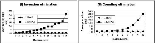
Figure 3: (I) Average run time for answering query P(death) from {epidemic 0.55, if epidemic then sick(X) 0.7 else 0.01, if sick(X) then death 0.55}, which requires inversion elimination only. (II) Average run time for answering query P(r) from p(X)∧p(Y )∧r 0.51, X ̸ = Y , which requires counting elimination.

and uses counting elimination only. In both cases propositional inference starts taking very long before any noticeable variation in lifted inference run times.

6 Discussion

We presented and showed the correctness of a lifted firstorder probabilistic inference algorithm, the first one to our knowledge that covers all cases in its intended language. This allows expressive representations whose inference is made much cheaper by abstracting away from specific instances of random variables and dealing instead with whole classes of them at once. We believe this type of algorithm will be essential to the development of large and expressive probabilistic systems, especially when the particular model is not known in advance and a general and automatic approach is necessary.

We presented two ways of eliminating variables: inversion and counting elimination. Counting elimination is potentially much more expensive than inversion elimination, but we expect its occurrence in practical problems to be low; in any case, we believe that much better counting arguments exist. Investigating them is an interesting line for further research.

Many other interesting directions remain to be taken. A very natural extension would be to allow non-ground queries that produce not only probabilities but also bindings for logical variables. Also, the algorithm can be adapted, in a way similar to [Pfeffer and Koller, 2000], in order to work with infinite models, allowing for richer constraint languages where constraints may have infinite solutions, as for example those with function symbols. This is also related to Constraint Logic Programming [Van Hentenryck, 1989]. Given the complexity of the language, approximation schemes will be very important for practical applications; counting elimination seems a particularly good place to start given its relatively high cost but also regularity. Techniques from theorem proving will be particularly useful when models with a large number of parfactors are necessary and one has to apply them wisely. A complexity study is also necessary for, among other things, guiding the choice of efficient elimination orderings.

Much of the gain in performance from a lifted algorithm comes from the presence of a large number of indistinguishable objects in the domain, that is, objects about which we have exactly the same knowledge. It has been argued ([Chavira et al., 2004]) that this does not occur often in practical applications. However, the current work simply provides a base for extensions with other important benefits. In an approximate inference setting, for example, the notion of indistinguishable objects is replaced by that of objects about which there is approximately the same knowledge (according to the current approximation factor), a much more practical situation. For non-ground queries, a problem of great practical interest, lifted inference is much more suitable, since the answers to such queries may be lifted themselves.

Acknowledgments

We would like to thank Vasin Punyakanok, Dav Zimak and the anonymous reviewers for their helpful comments. This research was supported by the Advanced Research and Development Activity (ARDA)'s Advanced Question Answering for Intelligence (AQUAINT) Program, by NSF grant ITR-IIS-0085980 and DAF Air Force Research Laboratory grant FA8750-04-2-0222 (DARPA REAL program).