
First-order probabilistic inference
Proceedings of the Eighteenth International Joint Conference on Artificial Intelligence. Pages 985-990.
© 2003 International Joint Conferences on Artificial Intelligence
Abstract
There have been many proposals for first-order belief networks (i.e., where we quantify over individuals) but these typically only let us reason about the individuals that we know about. There are many in stances where we have to quantify over all of the individuals in a population. When we do this the population size often matters and we need to reason about all of the members of the population (but not necessarily individually). This paper presents an algorithm to reason about multiple individuals, where we may know particular facts about some of them, but want to treat the others as a group. Combining unification with variable elimination lets us reason about classes of individuals without needing to ground out the theory.
- Bacchus, F. [1990]. Representing and Reasoning with Uncer- tain Knowledge, MIT Press, Cambridge, Massachusetts.
- PROBABILISTIC INFERENCE
- Breese, J. S. [1992] . Construction of belief and decision net- works, Computational Intelligence 8(4): 624-647.
- Buntine, W. L. [1994]. Operations for learning with graph- ical models, Journal of Artificial Intelligence Research 2: 159-225.
- Chang, C. L. and Lee, R. C. T. [1973]. Symbolic Logical and Mechanical Theorem Proving, Academic Press, New York.
- Dfez, F. J. and Galan, S. F. [2002]. Efficient computation for the noisy max, International Journal of Intelligent Systems p. to appear.
- Halpern, J. Y. [1990]. An analysis of first-order logics of probability, Artificial Intelligence 46(3): 311-350. IJCAI
- Horsch, M. and Poole, D. [1990] . A dynamic approach to probabilistic inference using Bayesian networks, Proc. Sixth Conference on Uncertainty inA/, Boston, pp. 155- 161.
- Jaeger, M. [2000] . On the complexity of inference about probabilistic relational models, Artificial Intelligence 117: 297-308.
- Kersting, K. and De Raedt, L. [2000]. Bayesian logic pro- grams, Linkoping Electronic Articles in Computer and Information Science 5(34). URL: http://www. ep.liu.se/ea/cis/2000/034/ Link
- Koller, D. and Pfeffer, A. [1998]. Probabilistic frame-based systems, AAA/-98, AAAI Press, Madison, Wisconsin.
- Pasula, H. and Russell, S. [2001]. Approximate inference for first-order probabilistic languages, /JCA/-01 , Seattle, WA, pp. 741-748. IJCAI
- Pearl, J. [1988]. Probabilistic Reasoning in Intelligent Sys- tems: Networks of Plausible Inference, Morgan Kauf- mann, San Mateo, CA.
- Pfeffer, A., Koller, D., Milch, B., and Takusagawa, K. [1999]. SPOOK: A system for probabilistic object- oriented knowledge representation, UAI-99, Stockholm, Sweden, pp. 541-550.
- Poole, D. [1993]. Probabilistic Horn abduction and Bayesian networks, Artificial Intelligence 64(1): 81-129.
- Poole, D. and Zhang, N. L. [2003] . Exploiting contextual inde- pendence in probabilistic inference, Journal of Artificial Intelligence Research 18: 263-313.
- Robinson, J. A. [1965]. A machine-oriented logic based on the resolution principle, Journal A CM 12( 1 ): 23-41.
- Wellman, M., Breese, J. and Goldman, P. [1992]. From knowl- edge bases to decision models, Knowledge Engineering Review 7(1): 35-53.
- Zhang, N. and Poole, D. [1996]. Exploiting causal indepen- dence in Bayesian network inference, Journal of Artifi- cial Intelligence Research 5: 301-328.
References were extracted automatically from the PDF and may contain errors.
Full text extracted automatically from the PDF; figures, tables and equations may differ. The PDF is the version of record.
1 Introduction
Belief networks or Bayesian networks [Pearl, 1988] are a pop ular representation for independencies amongst random vari ables. They are, however zeroth-order representations; to rea son about multiple individuals, we have to make each property of each individual into a separate node.
There have been proposals to allow for ways to lift belief networks to a first order representation. The first tradition [Breese, 1992; Horsch and Poole, 1990; Wellman, Breese and Goldman, 1992] essentially allowed for parameterized belief networks, which could be grounded for each individual. The second tradition [Poole, 1993; Koller and Pfeffer, 1998; Pfef fer, Koller, Milch, and Takusagawa, 1999] allowed for richer first order probabilistic representations that have belief net works as special cases. In all of these the only individuals assumed to exist are those that we know about.
There are many cases where we want to reason about a set of individuals as a group. We'd like avoid explicit reasoning about each individual separately. There was a great advance in theorem proving in the 1960s with the invention of of reso lution and unification [Robinson, 1965]. The big advance was that doing resolution on clauses that contain free variables implements a potentially unbounded number of resolutions on the grounded representation. The goal of the current work is to allow for similar savings in probabilistic reasoning.
Probabilistic reasoning is more challenging than logical rea soning for a number of reasons:
- We have to use all of our information when making a probabilistic inference; new information can change old conclusions.
- We don't want to double count evidence. If we have some probabilistic information about all people and we use it for one particular individual, say Fred, then we can't reuse that information for Fred.
- There are cases where the size of the domain affects the probability. In the example developed below, determin ing the probability that a person is guilty of a particular crime depends on the population; the population size af fects the number of other people who could be guilty.
The following example shows why we may need to reason about the individuals we don't know about as well as the indi viduals we do know about and shows why we need to consider population size.
Example 1 A person in a town was seen committing a crime. This person had the same (unusual) hair colour and car colour as Joe (both purple) and the person was very tall and we know Joe has big feet (and being tall is correlated with having big feet). What is the probability that Joe is guilty? We need to model the probabilities of the observations and their depen dence, which would lead us to consider belief networks as a representation. The probability Joe is guilty also depends on the population. If the population of the town is very small then he is probably guilty (as it is unlikely there is anyone else fitting this description). If the town was a city containing a large number of people then he is probably innocent (as we would expect many other people to also fit this description).
This example points to a number of features that have been ignored in first-order probabilistic models. Not only do we need to take population sizes into account but we need to be able to reason about the individuals we know about as well as the individuals who we know exist, but we don't know anything particular about. We don't have to ground out our theory and reason about millions of people in a city separately, but we also cannot ignore the relevant information about the people we know something about.
2 Representation
We assume that the domain is represented as a parametrized belief network, where the nodes are parametrized with domain-restricted types (or populations). Such an idea has been explored previously [Horsch and Poole, 1990; Kersting and De Raedt, 2000], and is similar to the plates of Buntine [ 1994]. We will not dwell on the semantics in this paper. We just assume that the program means the grounding: the sub stitution of constants for each individual in the domain of a parameter.
This paper is explicitly Bayesian. In terms of the first-order probability of Halpern [1990], the probabilities are all degrees of belief, not statistical assertions about proportions of a pop ulation. We are not quantifying over random individuals (as does Bacchus [ 1990]), but over all individuals (i.e., with stan dard universal quantification). All of the individuals about which we have the same information have the same probabil ity. It is this property that we exploit computationally.
This paper is built on two different traditions, namely that of logic programming and theorem proving on one side and that of probabilistic reasoning on the other side. Unfortu nately they use the same terms or notations (e.g., "variable", "domain","=") for very different things (or at least they are used in very different ways in this paper). In order to avoid confusion, we use neutral terms, but use the traditions of the different communities as appropriate.
A population is a set of individuals. A population corre sponds to a domain in logic. The cardinality of the population is called the population size. For example, the population may be the set of people living in Vancouver, and the popula tion size is 2 million people. The population size can be finite or infinite.
We allow for random variables to be parametrized, where parameters start with an upper case Jetter and constants start with a lower case Jetter. Parameters correspond to logical vari ables (e.g., as a variable in Prolog). All of the parameters are typed with a population. A parametrized random variable is of the formf(t1, ... , tk) where/ is a functor (either a function symbol or a predicate symbol) and each t; is a parameter or a constant. Each functor has a set of values called the range of the functor.
Examples of parametrized random variables are hair _colour(X), likes(X, Y), likes(joe, X) or town_conservativeness (the latter being a functor of no argu ments), where hair _colour, likes and town_conservativeness are functors.
Given an assignment of a constant to each parameter, a parametrized random variable represents a random vari able. For example, suppose hair colour has range {black, blond, red, grey, purple, orange, none, multicoloured}. Then hair _colour(sam) is a random variable with domain {black, blond, red, grey, purple, orange, none, multicoloured}. Thus a parametrized random variable represents a set of random variables, one for each parameter assignment. Different pa rameter assignments for the variables in a parametrized ran dom variable result in different random variables; for ex ample, hair _colourlfred) is a different random variable to hair _colour(joe).
A parametrized primitive proposition is an expression of the form t = v, which means that parametrized random variable t has value v. A parametrized proposition is built from the parametrized primitive propositions using the normal logical connectives.
A probabilistic assertion is of the form:
VX1 : d1, ... , vxk : dk; c-+ P(ai,B) = p where X; are parameters, d; are populations, C is a set of inequality constraints on X 1, ... , Xk. a and .B are parametrized propositions using only the parameters X I, ... , xk. p specifies a probability distribution over a . We omit the corresponding syntactic constructs when k = 0, C = {} or .B = true.
A parametrized belief network consists of
- a DAG where the nodes are parametrized random variables,
- an association of a population to each parameter,
- an assignment of a range to each functor,
- a set of probability assertions for each node given its parents.
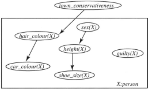
Example 2 To formalize Example 1, consider the parametrized belief network of Figure 1. Here we have shown it using the plates 1 [Buntine, 1994] as well as with parametrized random variables. We assume that the hair-colour of the different people are not independent; they depend on how conservative the town is. Associated with this network are conditional probabilistic assertions such as 2 :
P(conservative) = 0.7
'IX :person; P(guilty(X)) = 0.0000001
'IX: person; P(very_tall(X)Imale(X)) = 0.1
'IX :person; P(hair _colour(X)=purplel
conservative) = 0.001
If we knew as background knowledge that sam was an ex ception and has purple hair with probability 0.5, we would replace the last probabilistic assertion with:
'IX : person; X f= sam -+
P(hair _colour(X)=purplelconservative) = 0.001
1 Here we use plates just as a visual help; the real meaning is as probabilistic assertions. The plates get difficult to interpret when there are complex interactions between the parameters, but we can always interpret these as probabilistic assertions.
2 we use conservative as an abbreviation for town_conservativeness = conservative, male(X) as an abbreviation for sex(X) =male and very_tall(X) for height(X) = very_tall.
P(hair _colour(sam)=purple) = 0.5 (We will not use this in our continuing example).
A grounding of a parametrized belief network is a belief network that consists of all instances of the parametrized ran dom variables where each parameter is replaced by an in dividual in the population (or a ground term denoting that individual).
Intuitively, a parametrized belief network represents a huge belief network where the parametrized random variables are repeated for each individual in the population associated with the parameter for which the constraint is true. The above example, if there were 10,000 people, would represent a belief network with 60,001 nodes.
3 First order variable elimination
The problem that we consider is: given a parametrized belief network, a set of observations, and a (possibly parametrized) query to determine the conditional probability of the instances of a query given the observations. We assume that the evidence is a conjunction of existentially quantified parametrized prim itive propositions.
We consider the problem of parametric probabilistic infer ence in two stages: first, where every parameter that appears in the parents of a node also appears in the node and where the observations are variable-free. In this case, when we ground out the theory, each random variable only has a limited number of parents. In Section 3.5 we present the second case where we have parents that contain extra parameters; in this case we need a way to aggregate over populations. That section also considers existential observations and queries.
The algorithm is based on variable elimination, VE, [Zhang and Poole, 1996], where we eliminate the non-observed non query random variables one at a time. For first-order VE (FOVE) we eliminate all the instances of a functor at once 3 .
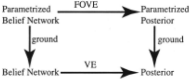
There is a strong relationship between this work and lifting in theorem proving [Chang and Lee, 1973]: given a ground proof procedure, construct a proof procedure with logical vari ables (or in our case with parametrized random variables). In general, correctness can be shown by proving that we get the same answer as if we first grounded the theory and then carried out variable elimination. See Figure 2.
3.1 Parametric Factors
In VE, a factor is the unit of data used during computation. A VE factor is a function from a set of random variables into a non-negative real number. The initial factors are the condi tional probabilities. The main operations are multiplying fac tors and summing out random variables from factors. After conditioning on the observed random variables and summing out the non-observed, non-query random variables, we can extract posterior probabilities from the remaining factors by multiplying them and normalizing the remaining factor.
In first-order variable elimination, we use a generalization of a factor where we want to treat the many instances of factors as a unit. We only instantiate parameters when we need to. In general we reason with all of the individuals (except the ones that we know extra information about) as a unit.
3 In general, we can potentially eliminate some instances of a func tor, but not necessarily all instances, and leave the other instances to be eliminated later. In this paper we will only do this when eliminat ing all instances except for a query instance.
A parametric factor or parfactor is a triple (C, V, t) where C is a set of constraints on parameters, V is a set of parametrized random variables and t is a table representing a factor from the random variables to the non-negative reals.
Intuitively the parametric factor represents all of the ground instances of the factor where the instantiation of the parameters satisfies the constraints.
Example 3 A parametric factor that represents one of the con ditional probability tables of Figure 1 is:
({}, {hair _colour(X) , conservativeness}, t)
where tis the table that represents a function from hair _colour and conservativeness into non-negative numbers. t is not in dexed by X . t looks like:
| hair _colour | conservativeness | Val |
|---|---|---|
| purple | conservative | 0.001 |
| purple | liberal | O.Ql |
| blue | conservative | 0.1 |
| blue | liberal | 0.05 |
When there are two instances of the same parametrized ran dom variable in V; in this case we need to mark the random variable in the table to distinguish these instances.
Example 4 Suppose that whether person X is a friend of Y depends on whether X likes Yand whether Y likes X. There are two distinct cases here, the first is when X = Y, in which case friends(X, Y) has one parent, and the second is when X f= Y, in which case friends(X, Y) has two parents. To represent this, we could use
( {}, {friends(X, X), likes(X, X)}, t1)
({X::/= Y}, lfriends(X, Y), likes1 (X, Y), likes2(Y, X)}, t2) where the subscripts in likes1 and likes2 represent different instances of likes in table t2. That is, t2 is a factor on friends, likes1 and likes2. When we eliminate all of the likes relation ships, we have to consider likes1 and likes2.
3.2 Splitting
The foundation of parametric variable elimination is the split ting operation. Splitting plays the analogous role to applying substitutions in theorem proving, except that we not only have to be concerned about the instance created, but also about the instances left over.
Definition 1 Suppose parametric factor ( C, V, t) contains pa rameter X. A split of ( C, V, t) on X = y, where y is either a constant or another parameter, and C does not contain X i= y (or y i= X), results in the two parametric factors:
where V[Xjy] is the same as V, but withy replacing every instance of X (i.e., we substitute y for X). The second para metric factor is called a residual parametric factor.
A substitution is of the form {XJ/tJ, ... , Xkftk} where the Xi are distinct variables and the ti are terms. We assume that all substitutions are in normal form: ti does not contain XJ for any i andj. The substitutions resulting from standard unification algorithms are in normal form [Chang and Lee, 1973]. If a substitution is in normal form, we get the same result from replacing each Xi by the corresponding ti sequentially (in any order) or in parallel.
Instead of just applying substitutions as in normal theorem proving, we need to split. The general idea is that whenever applying a substitution to a parfactor restricts the set of ground instances, we need to split the parfactor. We don't need to split when just renaming variables or substituting a value for a variable that doesn't appear in the parfactor.
We can split a parfactor ¢ on substitution (), by totally ordering the elements of the substitution 4 , {XJ/tJ, ... , Xkftk}, by carrying out the following procedure which results in a final instance of¢ and a set of residual parfactors:
For i from 1 to k
If Xi is a variable in ¢
then if ti is a variable in ¢ or ti is not a variable
then split¢ on xi = ti
else replace all occurrences of Xi by ti;
ti becomes a variable of¢.
Note that the final value of¢ is the same as if we had applied the substitution to ¢, but we also create residuals.
There is a close relationship between the splitting on equal ity in this paper and the splitting on the value of a variable in contextual variable elimination [Poole and Zhang, 2003].
3.3 Observations
When we observe a ground value, we carry out the analogous operation to VE. We project the tables onto the observed val ues. However we must first split to ensure that we only affect the appropriate ground variables.
Example 5 If we condition on the fact that Joe has purple hair, a purple car, and a shoe size of 12, we now reason separately about Joe than we do about the other individuals who can be treated as a group.
The parametric factor of example 3 becomes the two para metric factors:
({X i= joe}, {hair _colour(X), conservativeness}, t)
with the same t as above, and t' is t where we select hair _colour= purple and project onto conservativeness.
4 The total order does not affect the instance created but does affect which residuals are created.
3.4 Multiplying Parametric Factors
In VE, when we eliminate a variable, we multiply all of the factors that contain that variable then sum out the variable from the resultant factor.
As in variable elimination, we need to multiply the factors that contain the variable to be eliminated. In parametric vari able elimination, given two parametric factors, some instances may need to be multiplied, and some instances may not. Also, the dimension of the resulting factors can be different for dif ferent instances.
The product of two parametric factors, in general, results in a set of parametric factors. Intuitively, we keep splitting the parametric factors (and renaming parameters) until we can guarantee that we get parametric factors that, . if grounded, result in the same factors as if we were to first ground the factors and then multiply.
Determining which parfactors to multiply
Suppose there are two parfactors ¢1 = ( C1, {pJ} U V1, t1) and ¢2 = (C2, {p2} U V2, t2), with variables renamed to be differ ent, where PI and P2 are unifiable instances of p(XJ, .. . , Xk). where p is to be eliminated. Let() = mgu(p1, P2). We will split ¢1 on() and split ¢2 on(), putting all the residuals in the set <I> of all parfactors. All instances of the resulting non-residual parfactors would be multiplied in VE.
The following abstract example is designed to show what needs to be considered when multiplying parfactors. It isn't meant to be meaningful.
Example 6 Suppose we were to eliminate p and multiply the two parametric factors:
If we were to ground the parameters some of the instances of these would be multiplied in VE and some of them wouldn't. Unification finds the most general instances that are identical.
We unify p(X, a) and p(b, Z) resulting in the substitution () = {Xjb, Zja}.
We can split parametric factor ( 1) on () resulting in
Parametric factor (4) is a residual parametric factor. No in stance of parametric factor (4) ever needs to be multiplied by any instance of parametric factor (2) when eliminating p and doesn't participate further in the product.
Similarly, we can split (2) on () resulting in:
Parametric factor (6) is a residual factor and doesn't partici pate further in the elimination of p. All instances of (3) and (5) would be multiplied together when eliminating p(b, a) in variable elimination.
Determining the dimensionality of the product
In Example 6, all instances of parametric factors (3) and (5) would be multiplied if we were to ground parametric factors (1) and (2) and carry out VE. However, not all of the product factors have the same dimension; some have two different q instances, and some have one. We need to do more splitting to ensure that all of the products have the form of parametric factors.
Suppose we have parfactors ¢' = ( C', V', t') and ¢" = ( C", V", t") that need to be multiplied. If for all p' E V' and for all p" E V" , either p' and p" are identical or non-unifiable or if mgu(p', p") is incompatible with the constraints, we know that all instances of their product has the same dimension. If there is a p' E V' and p" E V" that are not identical but unify with mgu consistent with C' and C", we can split¢' and¢" on mgu(p', p") . The resulting instances and residuals either have identical instances of p' and p" or non-unifiable instances. We then multiply each instance created from ¢' by each instance created from ¢".
When we know all the instances ¢' = ( C', V', t') and ¢" = ( C" , V" , t") have the same dimension, we create the parfactor ( C' U C" , V' U V", t' ® t") where t' ® t" is the product of the tables for t' and t" where we maintain one dimension for each member of V' U V" . Thus, those members in common in V' and V" are treated as the same variable in the product, but those members that don't unify, even with the same functor, in V' and V" are treated as different variables in the product table.
Example 7 When we need to multiple parfactors (3) and (5), we notice that q(Y, c) and q(W, T) unify (with unifier {W / Y, T jc}). We thus split parametric factor (5) on T = c, and rename W to Y, replacing (5) with:
({Y f= d}, {p(b, a), q(Y, c), r(Y, c)}, t2} (7)({W ::/= d , T f= c}, {p(b, a), q(W, T), r(W, T)}, t2} (8)
We can now multiply parametric factors (3) and (7) producing:
({Y f= d}, {p(b, a), q(Y, c), r(Y, c), s(X, Y)}, t1 ® t2}
(9)
where t1 ® t2 is the product of factors . Parametric factor (9) represents all of the factors of dimension four created by multiplying factors that are instances of parametric factors (1) and (2).
We also multiply parametric factors (3) and (8) producing: ({W ::/= d, T f= c}, {p(b, a), q1 (Y, c), s(X, Y) , q2(W, T), r(W, T)}, ti ® t~) (10)where ti is the factor t1, but with q labelled as q1 and t~ is the factor t2, but with q labelled as q2. Thus ti ® t~ is a factor on p , q1, s, q2, r. Parametric factor (10) represents all of the factors of dimension five created by multiplying factors that are instances of parametric factors (1) and (2).
While this may seem very comflicated, remember that para metric factor (10) represents m (m - 1) 2 factors (assuming that all populations have size m). Even if m is 10, this is 8100 factors .
When we have multiplied all of the appropriate parfactors we are ready to sum out the variables being eliminated. We must remember that when we are eliminating p(XJ , ... , Xk), we are not just eliminating one random variable, but we are eliminating a number of variables equal to the product of the population sizes of X1, . .. , Xk . If some parameters only ap pear in the parametrized random variable that is being elimi nated, in the grounding we are multiplying the number of fac tors equal to the effective population size of those parameters.
To eliminate instances of p(XJ, ... , Xk) from multiset ci> of
parfactors: while there are parfactors ¢I = (CI , V1 , t1} and ¢2 = (C2 , V2, t2} in ci> (with variables renamed to be different) such that V1 = {p1} u v; and V2 = {p2} u V~ and PI and P2 are instances of p(XJ , . . . , Xk) that unify and() = mgu(p1, P2) is consistent with C1 and C2 { remove ¢1 and ¢2 from cl>; split ¢I on () with residuals going into cl>; split ¢2 on() with residuals going into cl> ; let <l>1 = {¢I}, <l>2 = {¢2}; while 3 ¢ ' = (C', {p'} U V', t') E c1> 1 and ¢" = (C", {p"} U V", t") E <l>2 and ¢' and ¢" are not identical and ()' = mgu(¢', ¢")and ()' is consistent with C' and C" { split¢' on ()' putting result and residuals in ci> 1 ; split¢" on ()' putting result and residuals in <l>2; } for every (C', V', t') E <l>1 and (C", V", t") E <l>2 { add (C' U C", V' U V" , t' ® t") to ci> } } for every (C, {p'} U V, t) E ci> where p' is an instance of p(XJ, .. . , Xk) { Jet m be the effective population size of the parameters in p' not in V replace (C, {p'} u V, t) with I C', V, o:=p' t)m\ in ci> where C' is C restricted to the parameters in V }The effective population size is the product of the populations of the parameters Jess the number excluded by the constraints. Thus we have to take each element in the table and put it to the power of the effective population size.
3.5 Aggregation over populations
When we have parameters in the parents of a node and not in the node itself, the number of parents grows with the popula tion size, and we need to specify how a node is a function of its parents. There are many possibilities, such as a node being the "logical or" of it's parents, the "logical and", the max of its parents, the average if its parents, true iff greater than k of its parents are true, or the vote of its parents (according to some voting scheme, for example when the majority wins), or some other function. Zhang and Poole [ 1996] give an analysis where there is an arbitrary associative and commutative oper ator between the parents. In order to make the presentation simpler, in this paper we assume that the operator is a logical "or" [Dfez and Galan, 2002]. It is straightforward to use the techniques of Zhang and Poole [ 1996] to extend this to other operators.
We can transform the problem into one of the form p(Z) with parents q(Z, X), where pis the "logical or", over all of the X values.
To eliminate q, we multiply all of the compatible clauses that contain q, and as we eliminate each q we accumulate the probability over the q's (as in [Dfez and Galan, 2002; Zhang and Poole, 1996]). The only difference is when there is a free (perhaps with inequality constraints) parameter in the X's. In this case we need to do the "or" over the effective population size. We can determine the effective population size by determining the effective population size of each free parameter by subtracting the number of excluded values from the population (e.g., if we have X f= a and X f= b with a population size of 10, we have an effective population size of 10-2=8) and multiplying by the effective populations of all of the free parameters.
If we have an effective population size of m and each one contributes a probability of p then, assuming they are all inde pendent, the probability that they are all false is ( 1 - p )m. So the probability that at least one is true (i.e., the logical "or") is 1- (1- p)m. If the effective population size is countably infinite, the probability that at least one is true is 1 if p > 0 and is 0 if p = 0.
However, we cannot assume the instances of the q's are in dependent. They are only dependent if they either have (1) a common ancestor in the grounding or (2) a common observed descendent. If we condition on the observation after elimi nating the q's, we can get around the second condition. The only way that the q's can have a common ancestor is if there is an ancestor that doesn't involve one of the parameters. If we make sure that we eliminate the q' s before we eliminate the common ancestors that separate the other common ancestors, then we can just use the equation above that assumes inde pendence. Effectively we are doing the logical "or" for each value of the ancestors, and we know they are independent for each value of the ancestors.
If we have an existential observation or query (e.g., condi tioning on the fact that someone who fits a certain description is guilty), we need to construct the "or" and either condition on or query the resulting node.
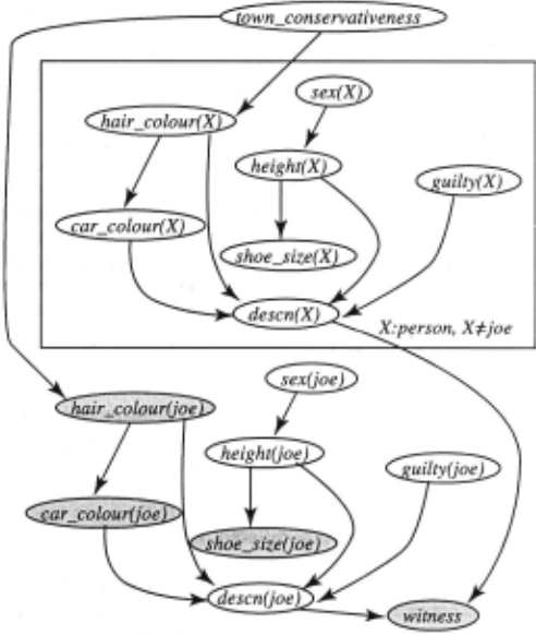
Example 8 Let's return to Example 1 (see Figure 1). Suppose that as well as observing the hair-colour, car-colour, and shoe size of Joe, we also observed that there exists a person who is guilty and fits a certain description of hair-colour, car-colour, height. This is depicted in Figure 4.
Suppose we want to compute whether Joe is guilty given Joe's hair-colour, car-colour and shoe size and given the wit ness description. We can first instantiate all of the observed random variables except the witness observation. This splits off joe as a special case. We can now eliminate all of the ran dom variables except for town_conservativeness, guilty(joe), descn(X) (for X =joe and X f= joe) and witness. This results in two parametric factors:
- ({}, {guilty(joe), descn(joe), conservativeness}, t1}
- ({X f=joe}, {descn(X), conservativeness}, t2}
We can now eliminate descn(X) for X f= joe and notice that the instances are independent given conservativeness. This results in the parametric factor:
({}, {guilty(joe), witness, conservativeness}, t3}
We can now sum out conservativeness and condition on witness and end up with a parametric factor
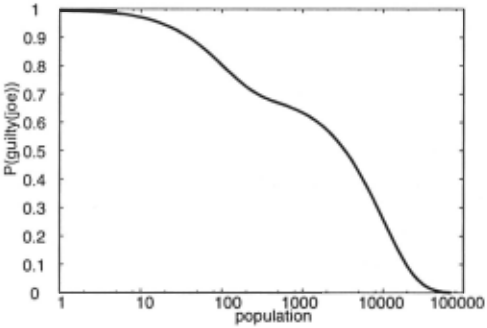
We can now determine the probability that Joe is guilty from normalising t4. If we were to carry out this computation leav ing the population as a parameter, the probability of guilty (joe) can be computed as a function of the population. We get a re sult that looks like Figure 5. The graph has this shape because it is the linear combination of exponential functions (for each value of town_conservativeness we have an exponential dis tribution).
4 Conclusion
This paper has made three main contributions:
- a way to do inference over populations without grounding out the theory and a way to use unification, where as well as the unifiers we also need to take into account the residuals;
- the idea that we need to take population size into account when we have aggregation over populations either as part of the model or as an observation; and
- a way to handle existential observations where we know someone exists but don't know who it is.
This paper extends the inference in object-oriented Bayesian networks [Pfeffer et a!., 1999] where the reasoning with generic class models corresponds to reasoning with free pa rameters in this paper. They do not use the power of unification as in this paper.
This paper contradicts the pessimistic conclusions of Jaeger [2000], but not the results. While in the worst case we may effectively ground the representation, in many cases we can do much better. How much we save in practice is still an open question.
There are still a number of open questions:
- What are good elimination orderings? We don't have to eliminate all instances of a functor at once.
- How to utilize other combination rules (apart from "or"). While the description here was in terms of noisy-or [Dfez and Galan, 2002] or inter-causal independencies [Zhang and Poole, 1996], the actual use of splitting is much closer to the work on contextual independence [Poole and Zhang, 2003].
- We are interested in combining the work in this paper with richer languages (e.g., Poole [ 1993 ]), where much of the power comes from mixing contextual independence and free variables and allowing for function symbols and recursion.
- It is also interesting to think about combining this with MCMC [Pasula and Russell, 2001], however it may not be straightforward because we are representing a set of individuals as a unit (and so are completely dependent), which may cause problems when we separate one indi vidual from the class and reason about that individual separately.
Acknowledgements
This work was supported by NSERC Research Grant OG P0044121 and The Institute for Robotics and Intelligent Sys tems. Thanks to Valerie McRae and Mark Paskin for valuable comments.
@inproceedings{ijcai2003p141,
  title     = {First-order probabilistic inference},
  author    = {Poole, David},
  booktitle = {Proceedings of the Eighteenth International Joint Conference on
               Artificial Intelligence, {IJCAI-03}},
  publisher = {International Joint Conferences on Artificial Intelligence},
  editor    = {Georg Gottlob and Toby Walsh},
  pages     = {985--990},
  year      = {2003},
  url       = {https://ijcai.org/proceedings/2003/141},
}
TY - CPAPER TI - First-order probabilistic inference AU - Poole, David T2 - Proceedings of the Eighteenth International Joint Conference on Artificial Intelligence, IJCAI-03 PB - International Joint Conferences on Artificial Intelligence PY - 2003 SP - 985 EP - 990 UR - https://ijcai.org/proceedings/2003/141 ER -Copied
Machine-readable versions of this paper, for tools and AI agents:





